LLM - Pre-training llms
LLM - Pre-training llms
Table of contents:
- LLM - Pre-training llms
Source:
Model Architecture
3 variance of the transformer model:
- encoder-only, encoder-decoder models, and decode-only.
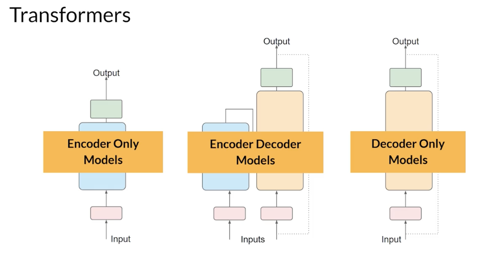
- Each of these is trained on a different objective, and so learns how to carry out different tasks.
- Autoencoding models: pre-trained using
masked language modeling, correspond to the encoder part of the original transformer architecture, and are often used withsentence classification or token classification. - Autoregressive models: pre-trained using
causal language modeling, make use of the decoder component of the original transformer architecture, and often used fortext generation. - Sequence-to-sequence models: use both the encoder and decoder part off the original transformer architecture. The exact details of the pre-training objective vary from model to model. often used for
translation, summarization, and question-answering
- Autoencoding models: pre-trained using
Encoder-only models
- Encoder-only models
- also known as
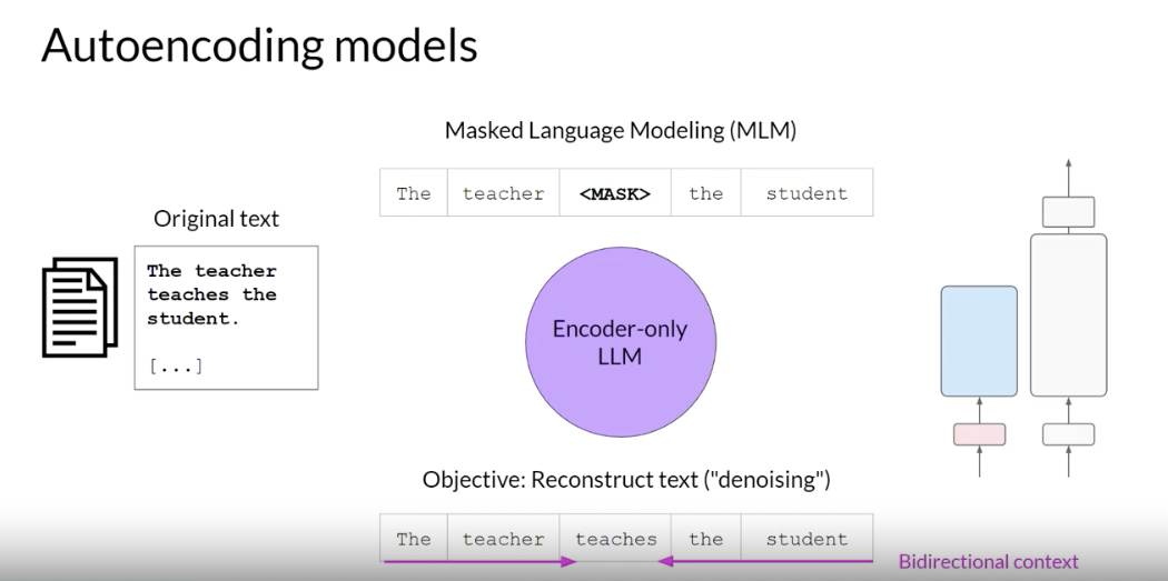
Autoencoding models - pre-trained using
masked language modeling. - This is also called a
denoising objective. - tokens in the input sequence are randomly mask, and the training objective is to predict the mask tokens in order to reconstruct the original sentence. .
Autoencoding models spilled bi-directional representations of the input sequence, meaning that the model has an understanding of the full context of a token and not just of the words that come before.
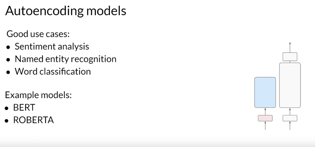
- Encoder-only models are ideally suited to task that benefit from this bi-directional </font> contexts.
- carry out sentence classification tasks, for example, sentiment analysis or token-level tasks like named entity recognition or word classification.
- autoencoder model: BERT and RoBERTa.
- also known as
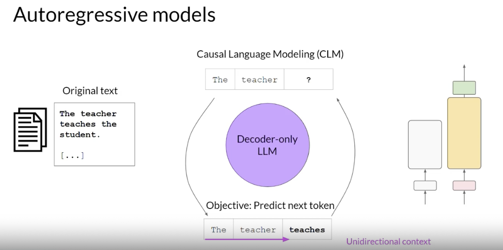
Decoder-only models
- decoder-only
autoregressive models,- pre-trained using
causal language modeling. - Here, the training objective is to predict the next token based on the previous sequence of tokens .
full language modeling- Decoder-based autoregressive models, mask the input sequence and can only see the input tokens leading up to the token in question.
- The model has no knowledge of the end of the sentence. The model then iterates over the input sequence one by one to predict the following token.
- In contrast to the encoder architecture, this means that the context is unidirectional </font>.
By learning to predict the next token from a vast number of examples, the model
builds up a statistical representation of language.- Models of this type make use of the decoder component off the original architecture without the encoder.
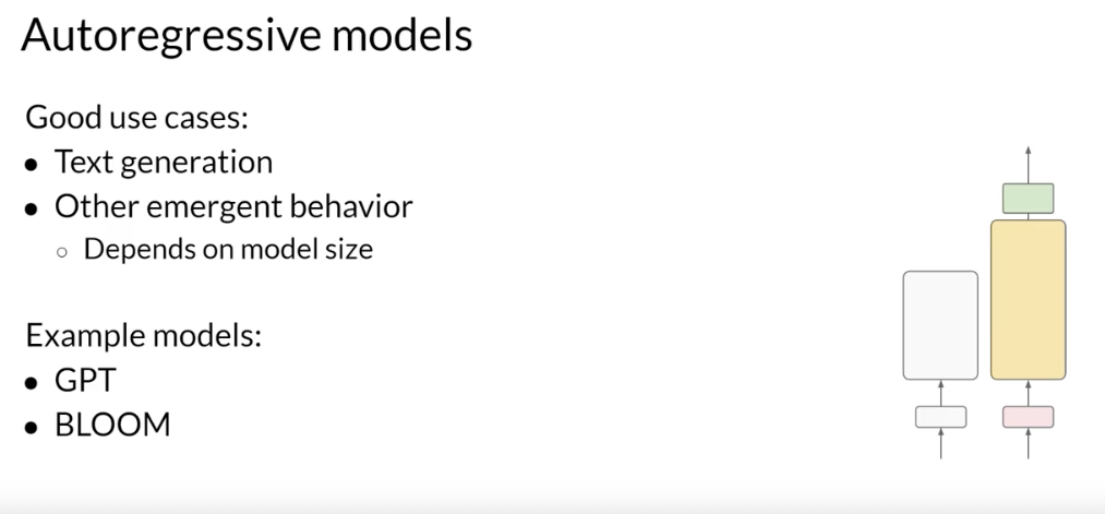
- Decoder-only models are often used for text generation , although larger decoder-only models show strong zero-shot inference abilities, and can often perform a range of tasks well.
- decoder-based autoregressive models: GBT and BLOOM.
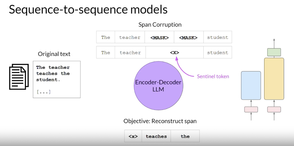
Encoder-Decoder models
- encoder-decoder models
- sequence-to-sequence model
- uses both the encoder and decoder parts off the original transformer architecture.
- The exact details of the pre-training objective vary from model to model.
- A popular sequence-to-sequence model T5,
- pre-trains the encoder using span corruption, which masks random sequences of input tokens. Those mass sequences are then replaced with a unique Sentinel token (x). .
- Sentinel tokens are special tokens added to the vocabulary, but do not correspond to any actual word from the input text
- The decoder is then tasked with reconstructing the mask token sequences auto-regressively. The output is the Sentinel token followed by the predicted tokens .
- pre-trains the encoder using span corruption, which masks random sequences of input tokens. Those mass sequences are then replaced with a unique Sentinel token (x). .
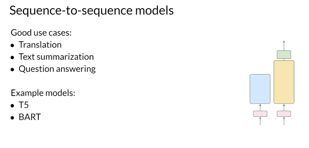
- use sequence-to-sequence models for translation, summarization, and question-answering . cases where you have a body of texts as both input and output.
- well-known encoder-decoder model: T5. BART
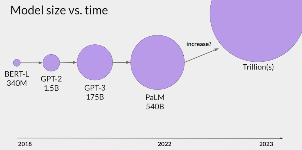
- the larger a model, the more likely it is to work as you needed to without additional in-context learning or further training.
- training these enormous models is difficult and very expensive, so that it may be infeasible to continuously train larger and larger models.
Pre-training llms
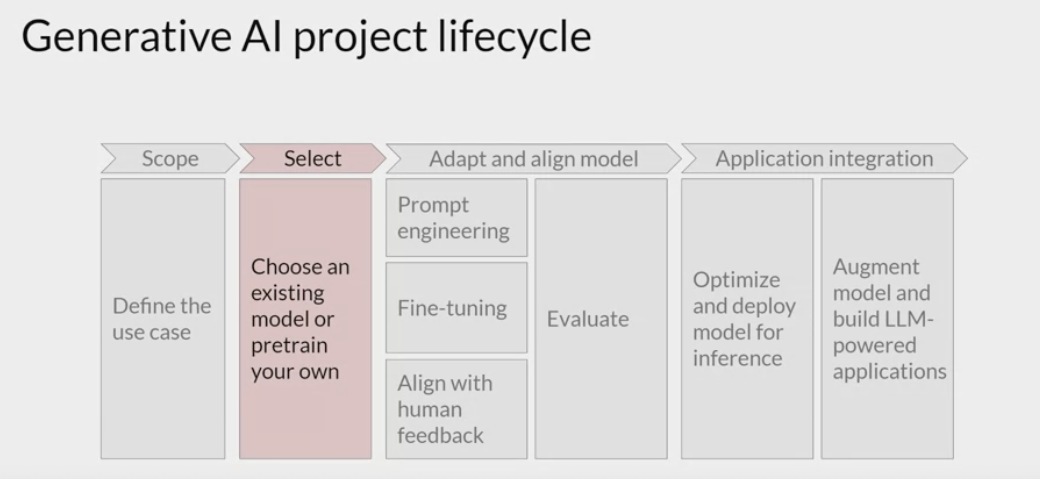
Once scoped out the use case, and determined how you’ll need the LLM to work within the application, the next step is to select a model to work with. the first choice will be to either work with an existing model, or train the own from scratch. There are specific circumstances where training the own model from scratch might be advantageous, and you’ll learn about those later in this lesson. In general, however, you’ll begin the process of developing the application using an existing foundation model.
The developers of some of the major frameworks for building generative AI applications like
Hugging FaceandPyTorch, have curated hubs where you can browse these models.Variance of the transformer model architecture are suited to different language tasks, largely because of differences in how the models are trained.
Pre-training objective
High-level look at the initial training process for LLMs.
This phase is often referred to as pre-training phase.
self-supervised learning step
LLMs encode a
deep statistical representationof language- the model learns from vast amounts of unstructured textual data .
- This can be gigabytes, terabytes, and even petabytes of text.
- This data is pulled from many sources and assembled specifically for training language models.
- the model internalizes the patterns and structures present in the language.
- These patterns then enable the model to complete its training objective, depends on the architecture of the model
During pre-training, the model weights get updated to minimize the loss of the training objective .
- The encoder generates an
embedding or vector representationfor each token.
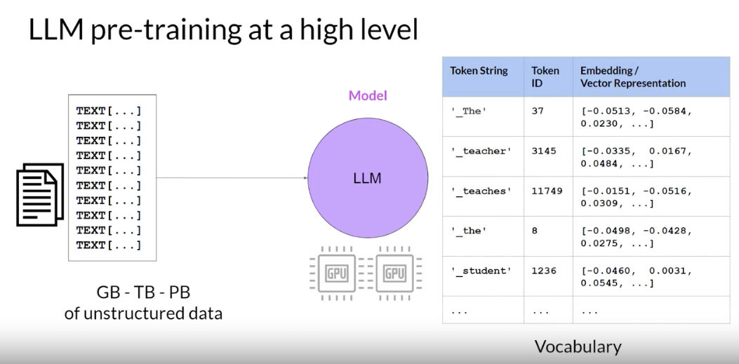
Pre-training also requires a large amount of compute and the use of GPUs.
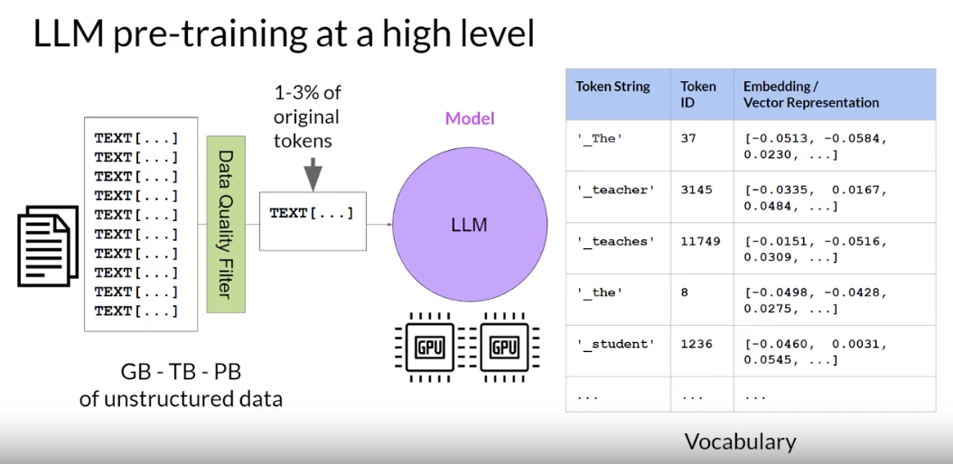
data quality curation
- when scrape training data from public sites such as the Internet, often need to process the data to increase quality, address bias, and remove other harmful content.
- As a result of this data quality curation, often
only 1-3% of tokensare used for pre-training. - You should consider this when you estimate how much data you need to collect to pre-train the own model.
Computational challenges of training LLMs
One of the most common issues you still counter when you try to train llms is running out of memory.
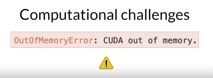
- on Nvidia GPUs, CUDA, short for
Compute Unified Device Architecture, is a collection of libraries and tools developed for Nvidia GPUs. - Libraries such as PyTorch and TensorFlow use CUDA to boost performance on metrics multiplication and other operations common to deep learning.
- You’ll encounter these out-of-memory issues because most LLMs are huge, and require a ton of memory to store and train all of their parameters.
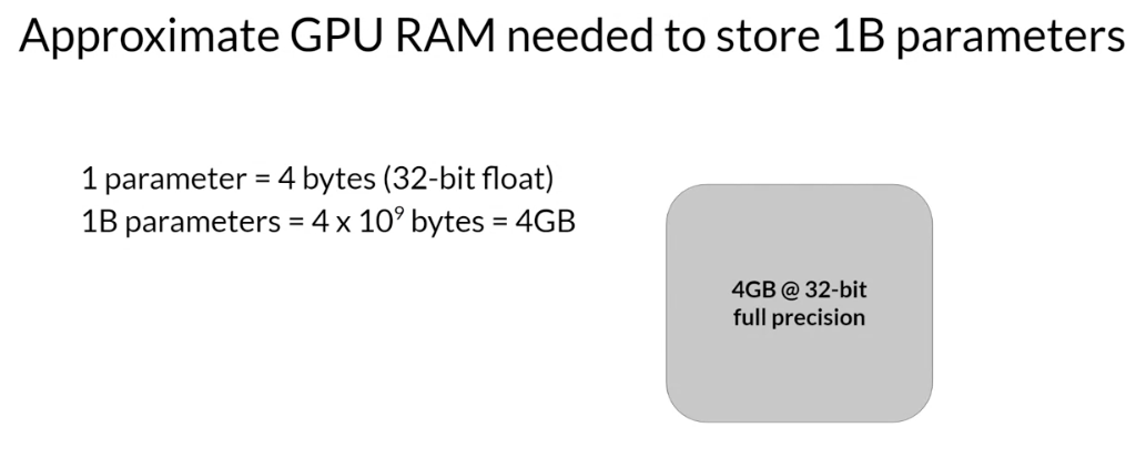
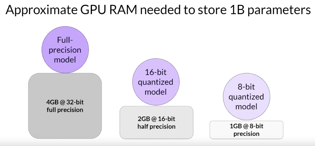
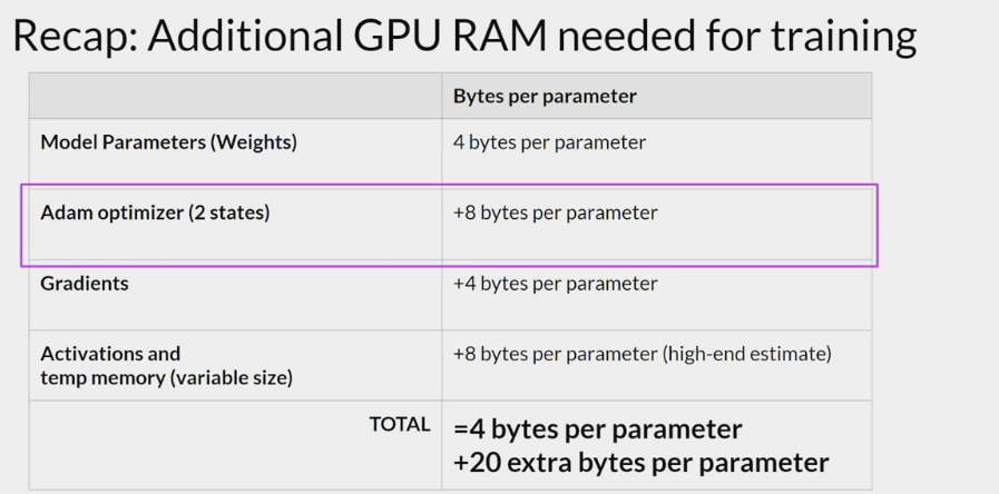
- A single parameter is typically represented by a
32-bit float, which is a way computers represent real numbers. A 32-bit float takes up four bytes of memory. - So to store
1B parameters -> four gigabyte of GPU RAM at 32-bit full precision.
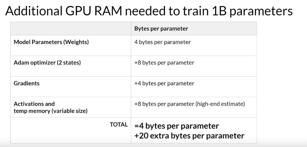
to train the model, you’ll have to plan for the memory to store the model weights + additional components that use GPU memory during training.
These include two Adam optimizer states, gradients, activations, and temporary variables needed by the functions. This can easily lead to 20 extra bytes of memory per model parameter.
- to account for all of these overhead during training, you’ll actually require approximately 6 times the amount of GPU RAM that the model weights alone take up.
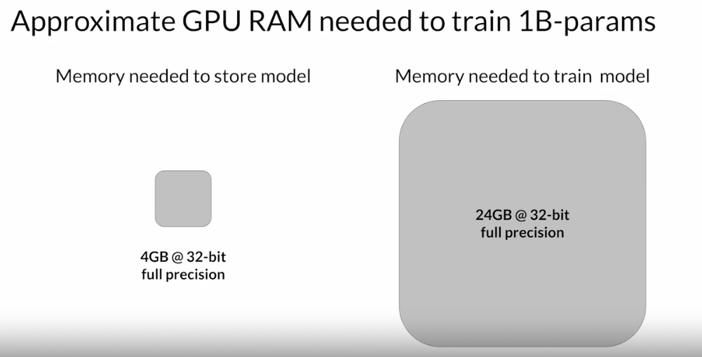
- To train a
1b parametermodel at 32-bit full precision -> approximately 24 gigabyte of GPU RAM.
To reduce the memory required for training
quantization
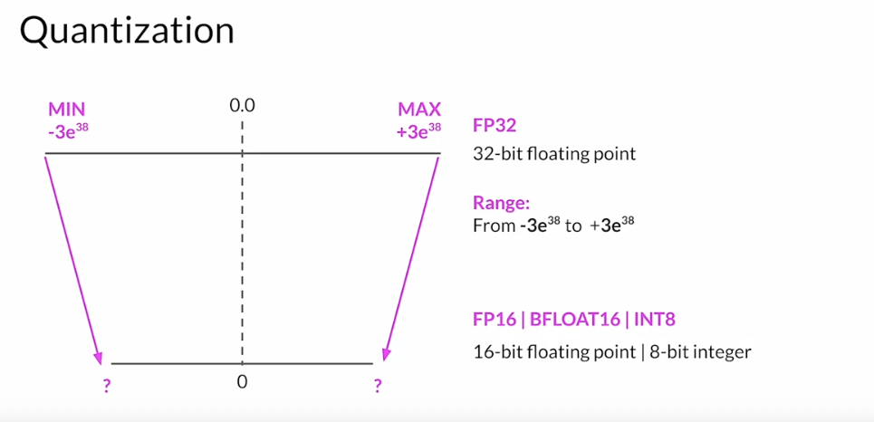
reduce the memory required to store the weights of the model by reducing their precision from
32-bit floating point numbersto16-bit floating point numbers, or8-bit integer numbers.Quantization statistically projects the original
32-bit floating point numbersinto a lower precision space, using scaling factors calculated based on the range of the original32-bit floating point numbers.- Let’s look at an example.
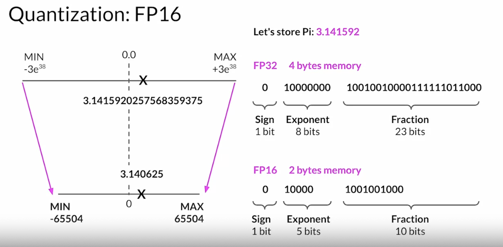

Suppose you want to store a PI to six decimal places in different positions.
- Floating point numbers are stored as a series of bits zeros and ones.
- The 32 bits to store numbers in full precision with FP32 consist of
- 1 bit for the sign where zero indicates a positive number, and one a negative number.
- 8 bits for the exponent of the number,
- 23 bits representing the fraction of the number. The fraction is also referred to as the mantissa, or significant. It represents the precision bits off the number.
If convert the 32-bit floating point value back to a decimal value, you notice the slight loss in precision.
if project this FP32 representation of Pi into the FP16, 16-bit lower precision space. The 16 bits consists of one bit for the sign, as you saw for FP32, but now FP16 only assigns five bits to represent the exponent and 10 bits to represent the fraction. Therefore, the range of numbers you can represent with FP16 is vastly smaller from negative 65,504 to positive 65,504. The original FP32 value gets projected to 3.140625 in the 16-bit space. Notice that you lose some precision with this projection. There are only six places after the decimal point now. You’ll find that
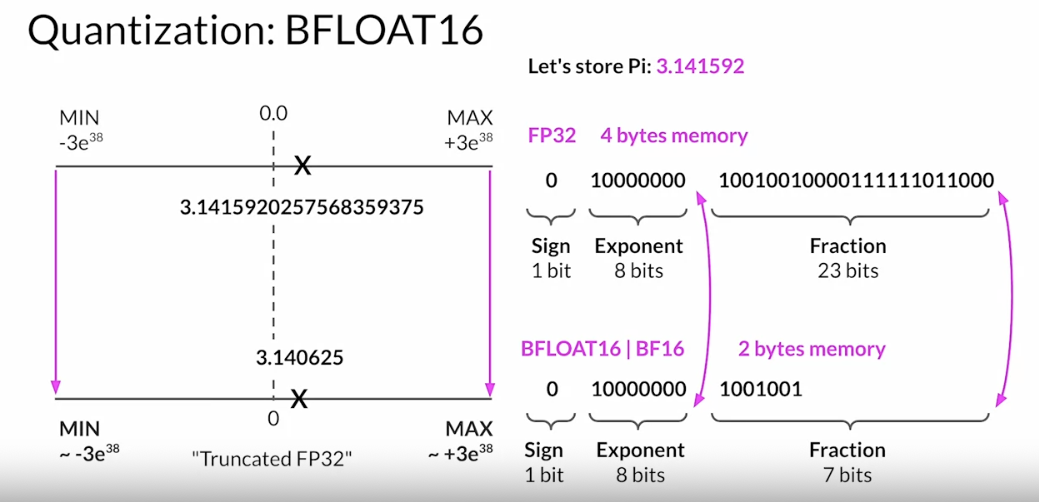
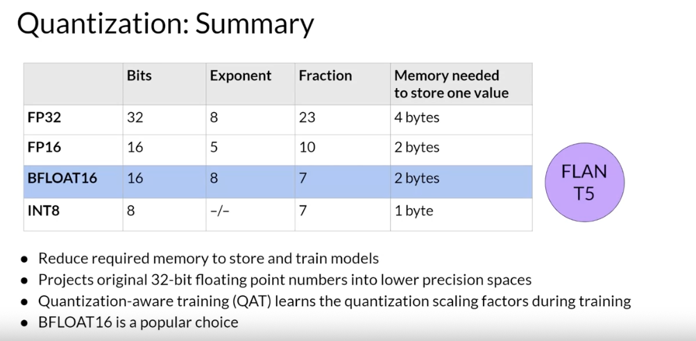
this loss in precision is acceptable in most cases because you're trying to optimize for memory footprint. Storing a value in FP32 requires four bytes of memory. In contrast, storing a value on FP16 requires only two bytes of memory, so with quantization you have reduced the memory requirement by half.The AI research community has explored ways to optimize16-bit quantization. One datatype in particular BFLOAT16, has recently become a popular alternative to FP16. BFLOAT16, short for Brain Floating Point Format developed at Google Brain has become a popular choice in deep learning. Many LLMs, including FLAN-T5, have been pre-trained with BFLOAT16. BFLOAT16 or BF16 is a hybrid between half precision FP16 and full precision FP32. BF16 significantly helps with training stability and is supported by newer GPU’s such as NVIDIA’s A100. BFLOAT16 is often described as a truncated 32-bit float, as it captures the full dynamic range of the full 32-bit float, that uses only 16-bits. BFLOAT16 uses the full eight bits to represent the exponent, but truncates the fraction to just seven bits.
This not only saves memory, but also increases model performance by speeding up calculations. The downside is that BF16 is not well suited for integer calculations, but these are relatively rare in deep learning.if you quantize Pi from the 32-bit into INT8 eight bit space. If you use one bit for the sign INT8 values are represented by the remaining seven bits. This gives you a range to represent numbers from negative 128 to positive 127 and unsurprisingly Pi gets projected two or three in the 8-bit lower precision space. This brings new memory requirement down from originally four bytes to just one byte, but obviously results in a pretty dramatic loss of precision.
- By applying quantization, you can
- reduce the
memory consumptionrequired to store the model parameters down to only two gigabyte using 16-bit half precision of 50% saving - further reduce the
memory footprintby another 50% by representing the model parameters as eight bit integers, which requires only one gigabyte of GPU RAM.
- reduce the
- the goal of quantization is to reduce the memory required to store and train models by reducing the precision off the model weights .
Quantization statistically projects the original
32-bit floating point numbersinto lower precision spaces using scaling factors calculated based on the range of the original 32-bit floats.Modern deep learning frameworks and libraries support quantization-aware training, which learns the quantization scaling factors during the training process.
- BFLOAT16 has become a popular choice of precision in deep learning as
it maintains the dynamic rangeof FP32, but reduces the memory footprint by half. in all these cases you still have a model with
1B parameters.Quantization will give you the same degree of savings when it comes to training. However, many models now have sizes in excess of 50B or even 100B parameters. Meaning you’d need up to 500 times more memory capacity to train them, tens of thousands of gigabytes. These enormous models dwarf the
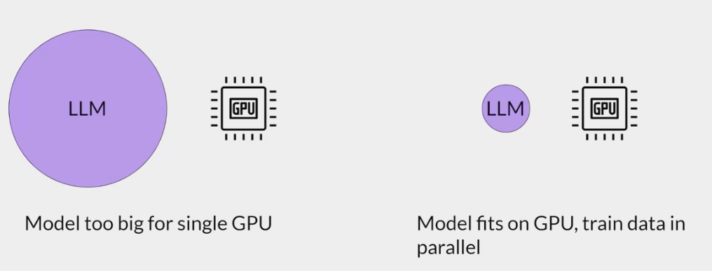
1B parametermodel we’ve been considering, shown here to scale on the left.- As modal scale beyond a few billion parameters, it becomes impossible to train them on a single GPU. you’ll need to turn to distributed computing techniques while you
train the model across multiple GPUs. This could require access to hundreds of GPUs, which is very expensive. - Another reason why you won’t pre-train the own model from scratch most of the time. However, an additional training process called fine-tuning, also require storing all training parameters in memory and it’s very likely you’ll want to fine tune a model at some point.
Efficient multi-GPU compute strategies
multi GPU compute strategies: distribute compute across GPUs, scale the model training efforts beyond a single GPU.
- when the model becomes too big to fit in a single GPU.
- or speed up the training even if the model does fit onto a single GPU.
scaling model training
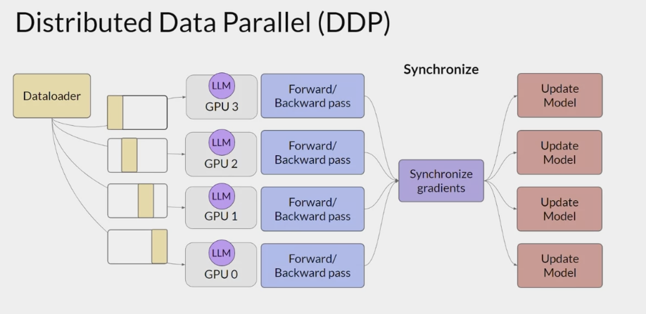
distribute large data-sets across multiple GPUs and process these batches of data in parallel.
- Data parallelism allows for the use of multiple GPUs to process different parts of the same data simultaneously, speeding up training time.
- Data parallelism is a strategy that splits the training data across multiple GPUs. Each GPU processes a different subset of the data simultaneously, which can greatly speed up the overall training time
.
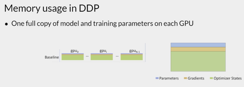
DDP (distributed data-parallel)
the model is still fits on a single GPU- A popular implementation of this model replication technique
- copy the model onto each GPU and sends batches of data to each of the GPUs in parallel.
- Each data-set is processed in parallel and then a synchronization step combines the results of each GPU, which in turn updates the model on each GPU, which is always identical across chips.
- This implementation allows parallel computations across all GPUs that results in faster training .
- Note that DDP requires that the model weights and all of the additional parameters, gradients, and optimizer states that are needed for training, fit onto a single GPU.
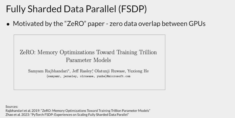
FSDP (Fully sharded data parallel)
models that are too big to fit on a single chip- allows scale model training across GPUs
when the model doesn't fit in the memory of a single chip. A popular implementation of modal sharding
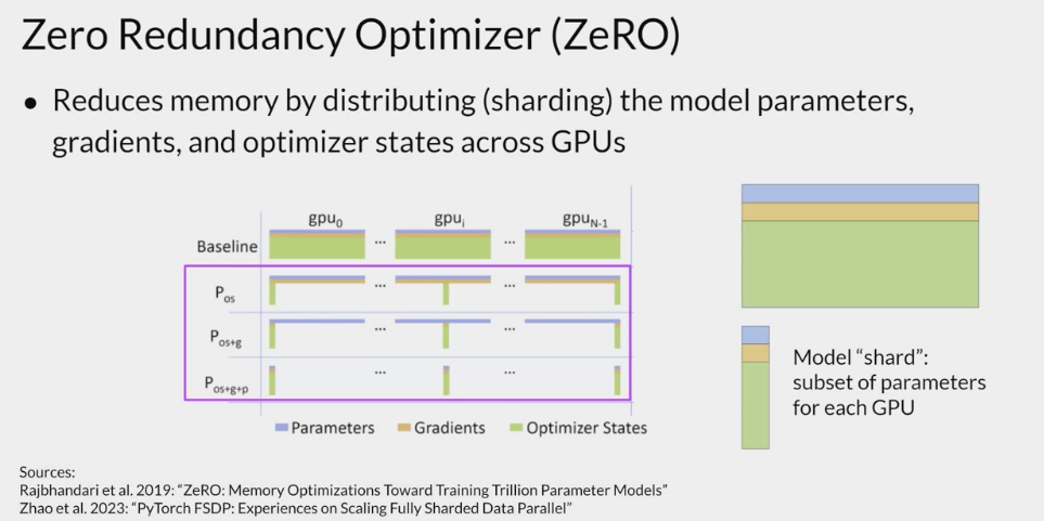
- FSDP is motivated by a paper published by researchers at Microsoft in 2019 that proposed a technique called
ZeRO.- ZeRO stands for zero redundancy optimizer
- the goal of ZeRO is to optimize memory by distributing or sharding model states across GPUs with ZeRO data overlap.
- FSDP allows reduce the overall GPU memory utilization.
- Optionally, you can specify that FSDP offloads part of the training computation to GPUs to further reduce the GPU memory utilization.
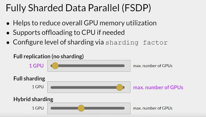
- To manage the trade-off between performance and memory utilization, you can configure the level of sharding using
FSDP charting factor.- full replication:
- sharding factor:1
- removes the sharding and replicates the full model similar to DDP.
- full sharding
- sharding factor:maximum number of available GPUs
- This has the most memory savings, but increases the communication volume between GPUs.
- hyper sharding
- Any sharding factor in-between
- full replication:
comparison
Recap all of the memory components required for tżraining LLMzs,
- the largest memory requirement was fożr the
optimizerstates, which take up twice as much space as the weights,- followed by
weightsand thegradieżnts.- Baseline:
- DDP:
- the parameters as this blue box,
- the gradients and yellow and
- the optimizer states in green.
- ZeRO:
- DDP
- One limitation off the model replication strategy is it keep a full model copy on each GPU, which leads to redundant memory consumption .
- storing the same numbers on every GPU.
- ZeRO
- eliminates this redundancy by distributing/sharding the model parameters, gradients, and optimizer states across GPUs instead of replicating them .
- the communication overhead for a sinking model states stays close to that of the previously discussed ADP.
- ZeRO offers 3 optimization stages.
- ZeRO Stage 1, shots only
optimizer states across GPUs, this can reduce the memory footprint by up to a factor of four. - ZeRO Stage 2 also
shots the gradients across chips. When applied together with Stage 1, this can reduce the memory footprint by up to eight times. - ZeRO Stage 3
shots all components including the model parameters across GPUs. 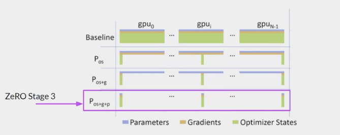
- ZeRO Stage 1, shots only
- When applied together with Stages 1 and 2, memory reduction is linear with a number of GPUs.
- For example, sharding across 64 GPUs could reduce the memory by a factor of 64.
- FSDP
- distribute the data across multiple GPUs as DDP, and also distributed or shard the model parameters, gradients, and optimize the states across the GPU nodes using one of the strategies specified in the ZeRO.
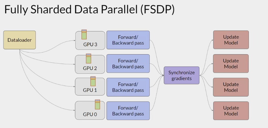
- forward and backward pass
- DDP: each GPU has all of the model states required for processing each batch of data available locally,
- FSDP: collect this data from all of the GPUs before the forward and backward pass.
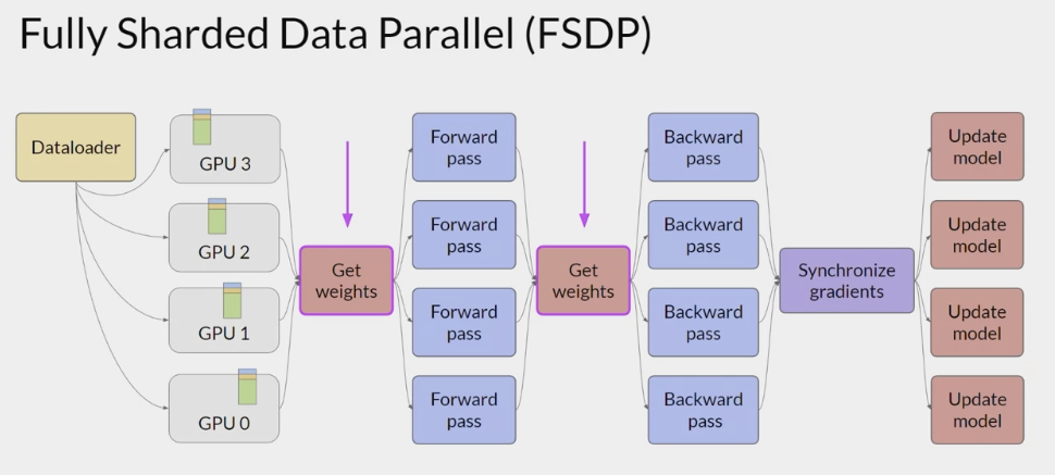
- Each CPU requests data from the other GPUs on-demand to materialize the sharded data into uncharted data for the duration of the operation.
- After the operation:
- release the uncharted non-local data back to the other GPUs as original sharded data
- or choose to keep it for future operations during backward pass, which requires more GPU RAM again,
- a typical performance vs memory trade-off decision.
- synchronizes gradients
- In the final step after the backward pass, FSDP is synchronizes the gradients across the GPUs in the same way as DDP.
Impact of using FSDP
- how FSDP performs in comparison to DDP measured in teraflops per GPU.
- These tests were performed using a maximum of 512 NVIDIA V100 GPUs, each with 80 gigabytes of memory.
one teraflop corresponds to one trillion floating-point operations per second.
- The first figure shows FSDP performance for different size T5 models.
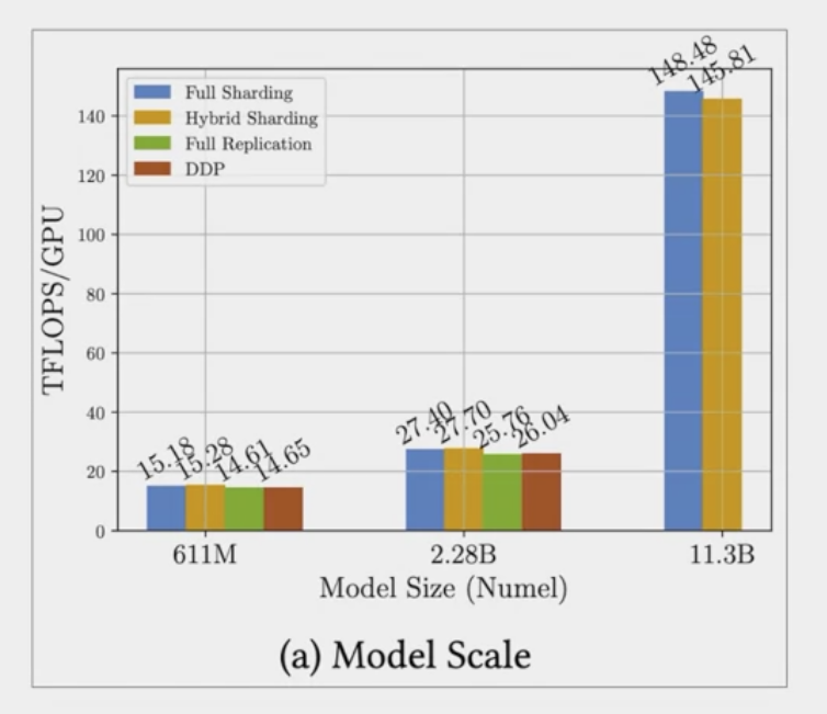
- You can see the different performance numbers for FSDP, full sharding in blue, hyper shard in orange and full replication in green, DDP performance is shown in red.
- For the first 25 models with 611 million parameters and 2.28 billion parameters, the performance of FSDP and DDP is similar.
- for model size beyond 2.28 billion, (such as 25 with 11.3 billion parameters), DDP runs into the out-of-memory error. FSDP on the other hand can easily handle models this size and achieve much higher teraflops when lowering the model’s precision to 16-bit.
- The second figure shows 7% decrease in per GPU teraflops when increasing the number of GPUs from 8-512 for the 11 billion T5 model, plotted here using a batch size of 16 and orange and a batch size of eight in blue.
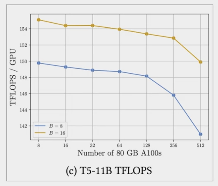
As the model grows in size and is distributed across more and more GPUs, the increase in communication volume between chips starts to impact the performance, slowing down the computation.
- In summary, this shows that you can use FSDP for both small and large models and seamlessly scale the model training across multiple GPUs.
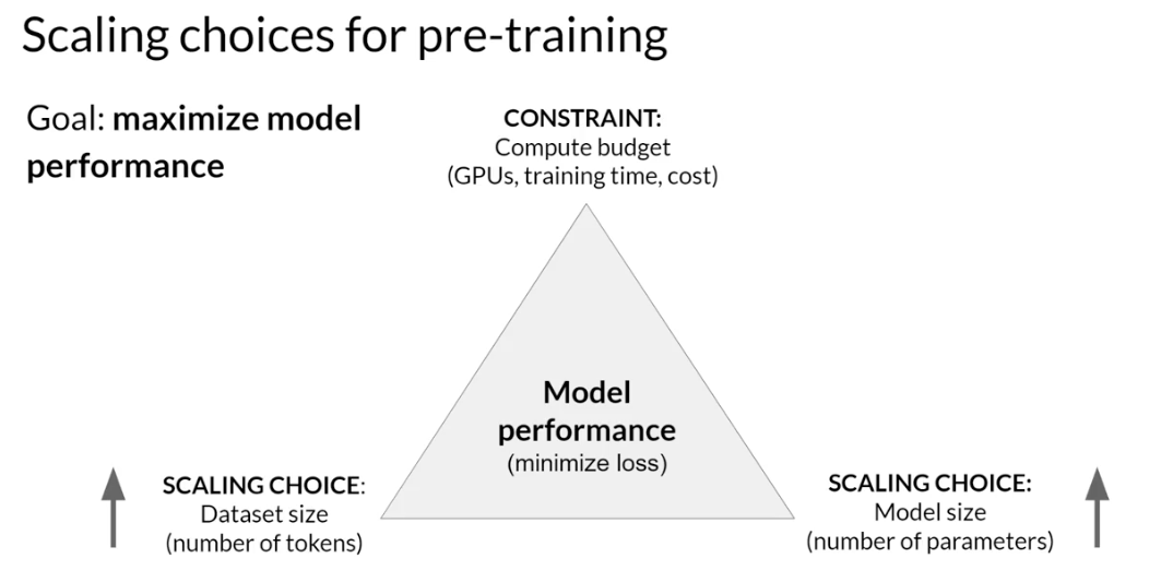
Scaling laws and compute-optimal models
- Increasing the dataset size and the number of parameters in the model can improve performance.
- The compute budget, including factors like available GPUs and training time, is an important consideration.
- The concept of a petaFLOP per second day is introduced as a measure of required resources for training models.
- A comparison is made between the compute resources needed for different variants of language models.
- There are trade-offs between training dataset size, model size, and compute budget.
- A power-law relationship is observed between these variables and model performance.
- The Chinchilla paper is mentioned, which explores the optimal number of parameters and training dataset size for a given compute budget.
- Many llms may be over-parameterized and under-trained.
- The Chinchilla model outperforms non-optimal models on downstream evaluation tasks.
- Smaller models are being developed that achieve similar or better results than larger models.
the relationship between model size, training, configuration and performance in an effort to determine just how big models need to be.
- the goal of pre-training:
- maximize the model's performance of its learning objective
- minimizing the loss when predicting tokens
- Two options you have to achieve better performance are
- increasing the size of the dataset
train the model on
- increasing the number of parameters
in the model.
- increasing the size of the dataset
In theory, you could scale either of both of these quantities to improve performance. However, consideration is the compute budget , factors like the number of GPUs you have access to and the time you have available for training models.
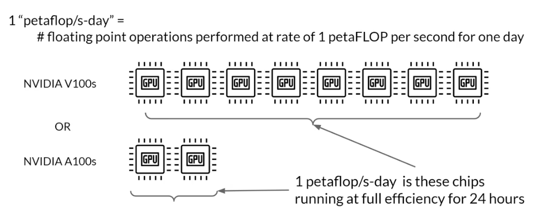
unit of compute that quantifies the required resources
petaFLOP
- A petaFLOP/s-day: measurement of the number of floating point operations performed at a rate of one petaFLOP per second, running for an entire day.
1 petaFLOP/s = one quadrillionfloating point operations per second.- in training transformers,
1 petaFLOP/s = 8 NVIDIA V100 GPUs, operating at full efficiency for one full day.
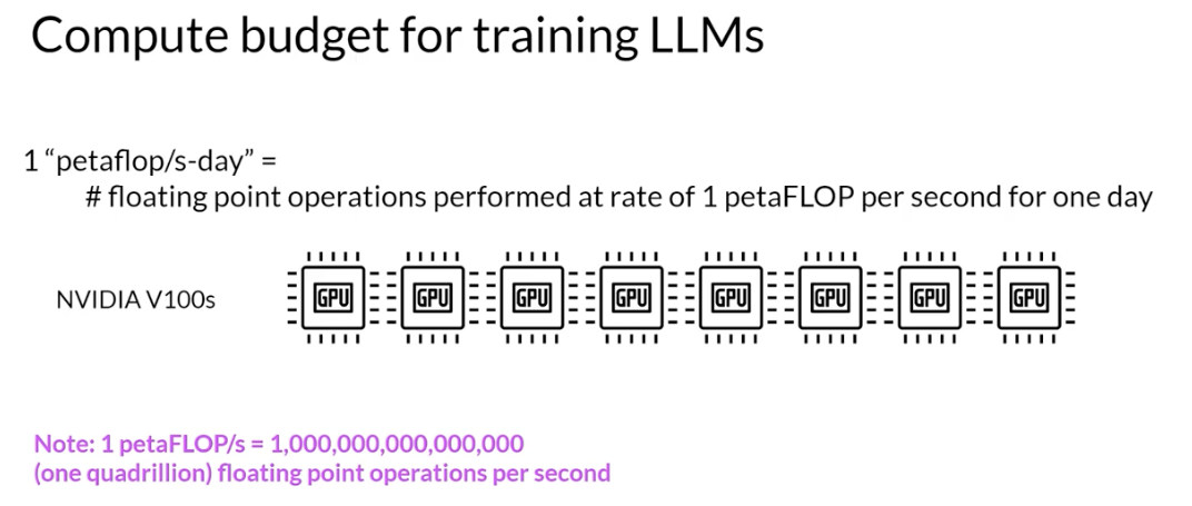
- If you have a more powerful processor that can carry out more operations at once, then a petaFLOP/s-day requires fewer chips.
- For example, 2 NVIDIA A100 GPUs give equivalent compute to the 8 V100 chips.
- huge amount of computers is required to train the largest models
- bigger models take more compute resources to train and generally also require more data to achieve good performance.
- they are actually well-defined relationships between these three scaling choices.
- compute budgets: this chart shows a comparison of
the petaFLOP/s-day required to pre-train different variance of Bert and Roberta (encoder only models), T5 (encoder-decoder model) and GPT-3 (decoder only model). 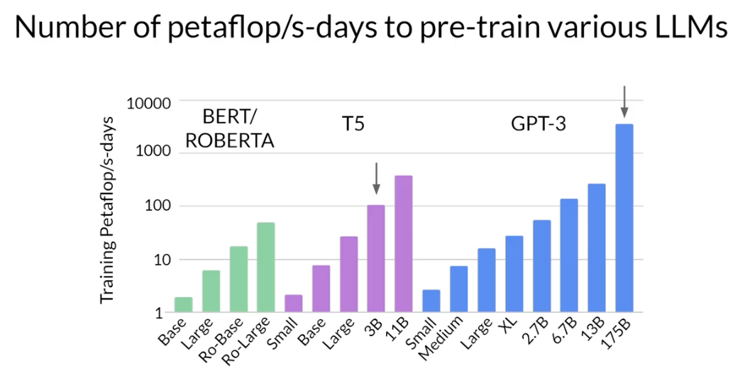
- The difference between the models in each family is the number of parameters that were trained
- the y-axis is logarithmic. Each increment vertically is a power of 10.
- T5 XL with three billion parameters required close to 100 petaFLOP/s-day.
- the larger GPT-3 175 billion parameter model required approximately 3,700 petaFLOP/s-day.
training dataset size, model size and compute budget
- Researchers have explored the trade-offs between training dataset size, model size and compute budget
.
larger numbers can be achieved by either using more compute power or, training for longer, or both.
- paper by researchers at OpenAI, explores
the impact of compute budget on model performance.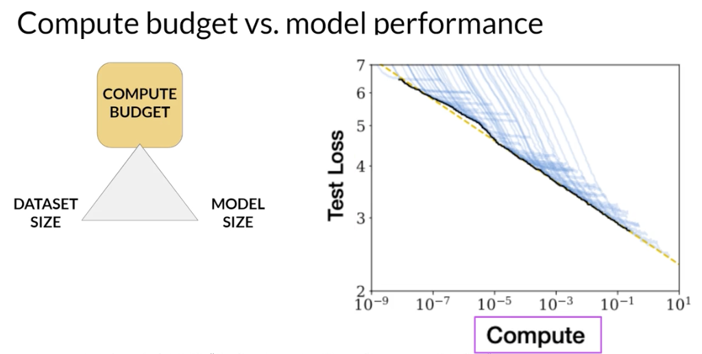
y-axis: test loss, consider as a proxy for model performance where smaller values are better.x-axis: the compute budget in units of petaFLOP/s-day.- Each
thin blue line: shows the model loss over a single training run. where the loss starts to decline more slowly for each run, reveals a clear relationship between the compute budget and the model’s performance.
- paper by researchers at OpenAI, explores
- power-law relationship: pink line.
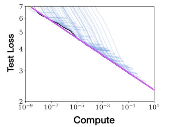
- a mathematical relationship between two variables, where one is proportional to the other, raised to some power.
- When plotted on a graph where both axes are logarithmic, power-law relationships appear as straight lines.
- The relationship here holds as long as model size and training dataset size don’t inhibit the training process -> you can just increase the
compute budgetto achieve better model performance.- In practice however, the compute resources available for training will generally be a hard constraint set by factors such as the
hardware you have access to, the time available for training and the financial budget of the project. - If you hold the compute budget fixed, the two levers you have to improve the model’s performance are
the size of the training datasetandthe number of parameters in the model. 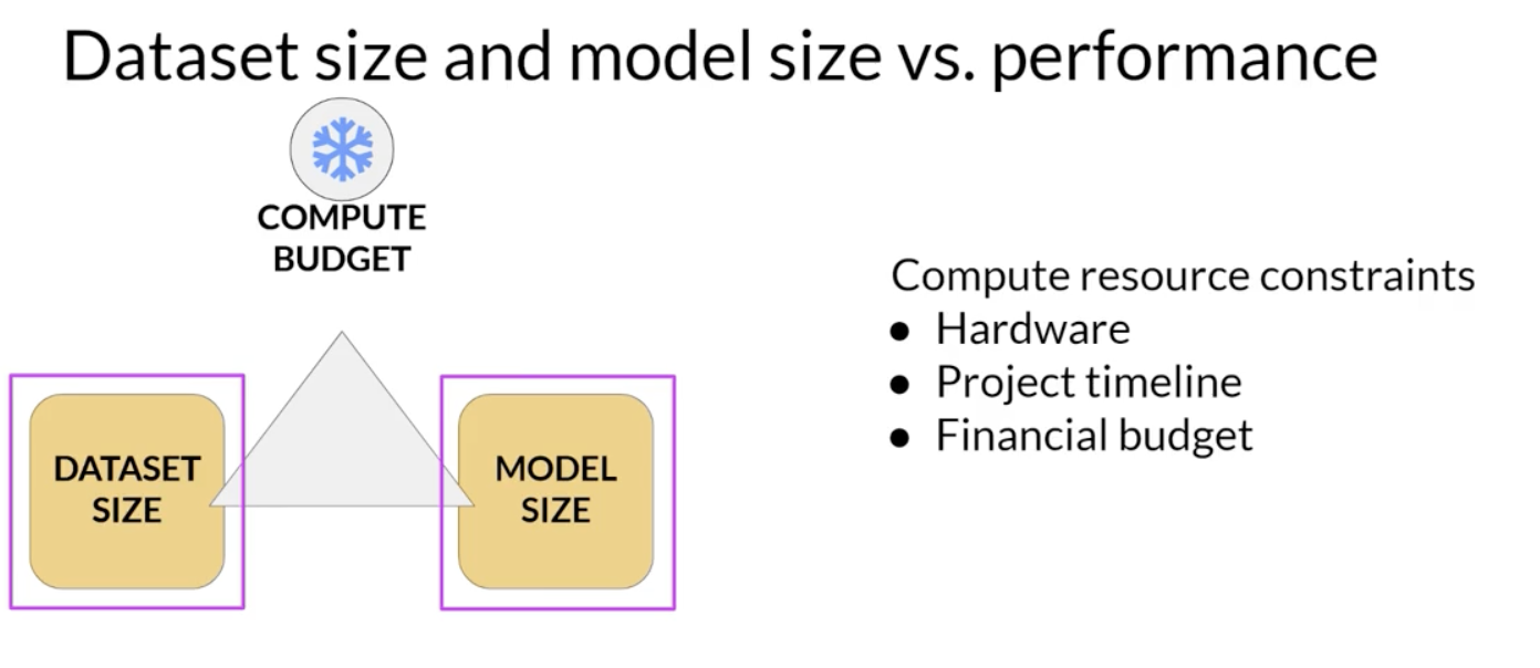
- In practice however, the compute resources available for training will generally be a hard constraint set by factors such as the
The OpenAI researchers found that these two quantities also show a power-law relationship with a test loss in the case where the other two variables are held fixed.
- when
compute budget and model sizeare held fixed and the size of the training dataset is vary.- The graph shows that as the volume of training data increases, the performance of the model continues to improve.
when
compute budget and training dataset sizeare held constant. Models of varying numbers of parameters are trained. As the model increases in size, the test loss decreases indicating better performance.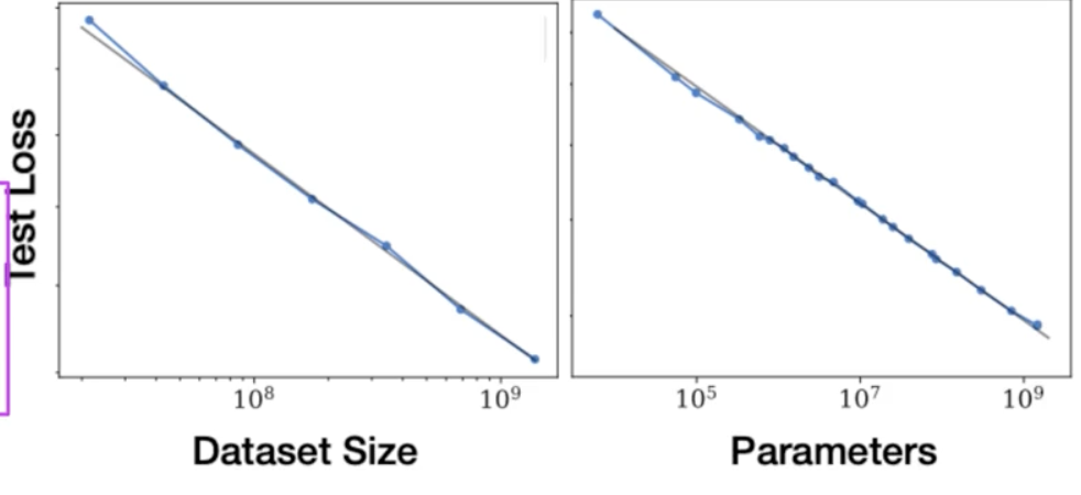
- when
ideal balance between these three quantities?
- Chinchilla paper
- paper published in 2022, a group of researchers led by Jordan Hoffmann, Sebastian Borgeaud and Arthur Mensch
- a detailed study of the performance of language models of various sizes and quantities of training data.
- The author’s name, the resulting compute optimal model, Chinchilla.
- The goal was to find the optimal number of parameters and volume of training data for a given compute budget
- The Chinchilla paper hints
- many of the 100 billion parameter llms like GPT-3 may actually be over parameterized
- they have more parameters than they need
to achieve a good understanding of language and under trained
- they would benefit from seeing more training data
.
- they have more parameters than they need
smaller models may be able to achieve the same performance as much larger ones if they are trained on larger datasets .
the optimal training dataset size for a given model is about 20 times larger than the number of parameters in the model.
- the compute optimal Chinchilla model outperforms non compute optimal models such as GPT-3 on a large range of downstream evaluation tasks.
- many of the 100 billion parameter llms like GPT-3 may actually be over parameterized
Chinchilla was determined to be compute optimal.
- a selection of models along with their size and information about the dataset they were trained on.
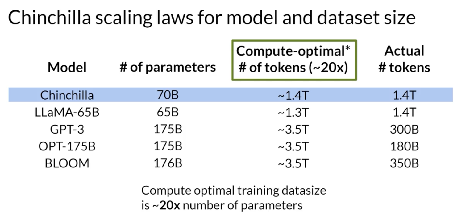
- For a 70 billion parameter model, the ideal training dataset contains 1.4 trillion tokens or 20 times the number of parameters.
- The last three models in the table were trained on datasets that are smaller than the Chinchilla optimal size. These models may actually be under trained.
- LLaMA was trained on a dataset size of 1.4 trillion tokens, which is close to the Chinchilla recommended number.
- paper published in 2022, a group of researchers led by Jordan Hoffmann, Sebastian Borgeaud and Arthur Mensch
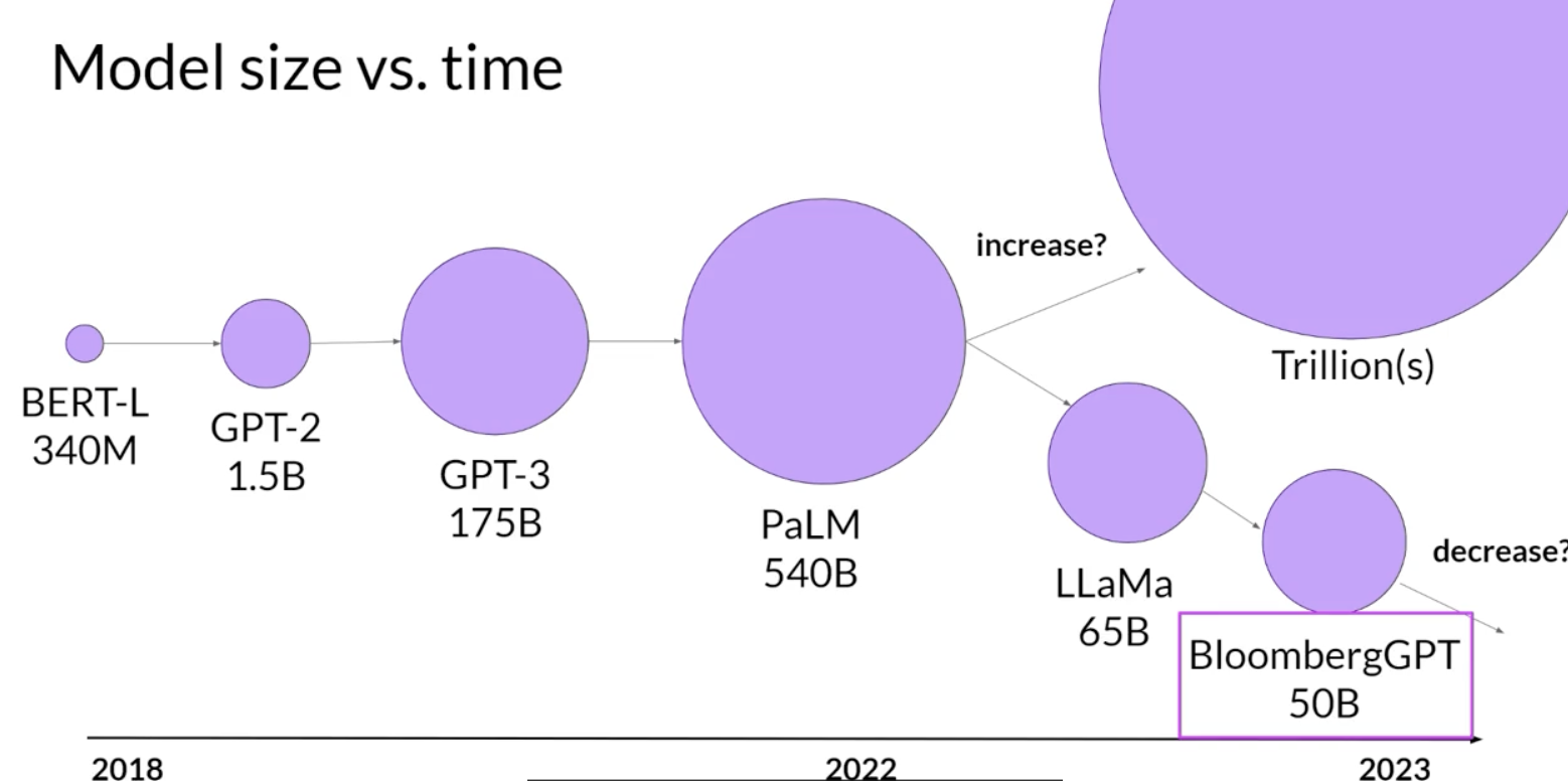
teams have recently started to develop smaller models that achieved similar/better results than larger models that were trained in a non-optimal way.
- expect to see a deviation from the bigger is always better trends of the last few years
Pre-training for domain adaptation
使用现有LLM的优点
- 在开发应用时,你通常会使用现有的LLM。这不仅节省了大量时间,还能更快地达到可行的原型阶段。然而,在某些情况下,你可能需要从头开始预训练自己的模型。这种情况通常出现在目标领域使用的词汇和语言结构在日常语言中不常见的情况下。
特殊领域的需求
- 例如,法律、医学、金融和科学等领域可能需要特定的术语和用法,这些词汇和结构在现有LLM的训练文本中可能不常见,因此模型可能难以理解或正确使用这些词汇。
If the target domain uses vocabulary and language structures that are not commonly used in day to day language.
Because models learn vocabulary and understanding of language through the original pretraining task. Pretraining the model from scratch will result in better models for highly specialized domains like law, medicine, finance or science.
- need to perform domain adaptation to achieve good model performance.
- words are rarely used outside of the legal world
- unlikely to have appeared widely in the training text of existing LLMs
- may not appear frequently in training datasets consisting of web scrapes and book texts
例如:
- 法律术语(如“mens rea”和“res judicata”)在法律之外几乎不会出现。
- 医学术语(如药物处方的缩写)在一般文本中也很少见。
- Some domains also use language in a highly idiosyncratic way.
- This last example of medical language may just look like a string of random characters, but it’s actually a shorthand used by doctors to write prescriptions. This text has a very clear meaning to a pharmacist, take one tablet by mouth four times a day, after meals and at bedtime.
BloombergGPT
- first announced in 2023 in a paper by Shijie Wu, Steven Lu, and colleagues at Bloomberg.
- an example of a LLM that has been pretrained for a specific domain, finance.
- The Bloomberg researchers chose to combine both finance data and general purpose tax data, pretrain a model that achieves Bestinclass results on financial benchmarks. While also maintaining competitive performance on general purpose LLM benchmarks.
the researchers chose data consisting of 51% financial data and 49% public data.
- tradeoffs
- These two graphs compare a number of LLMs, including BloombergGPT, to scaling laws that have been discussed by researchers.
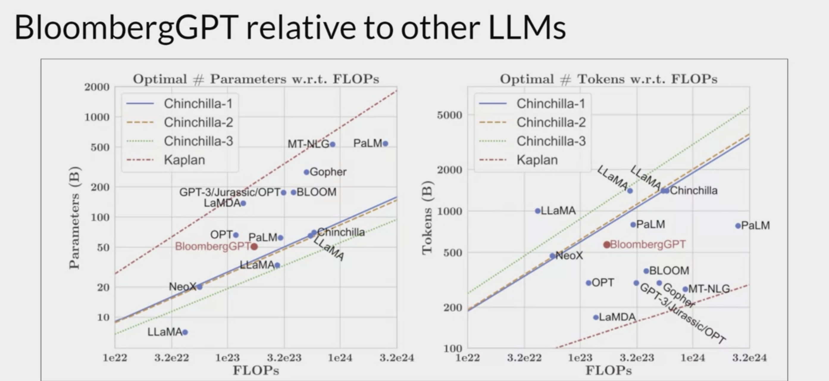
- On the left, the diagonal lines trace the optimal model size in billions of parameters for a range of compute budgets.
On the right, the lines trace the compute optimal training data set size measured in number of tokens.
- 在模型大小方面,BloombergGPT大致遵循Chinchilla的方法,对于1.3百万GPU小时的计算预算(约2.3亿petaFLOP),参数数量接近最优。
- 在训练数据集大小方面,由于金融领域数据的有限可用性,实际使用的训练数据(5690亿个词元)低于Chinchilla建议的值。
Comments powered by Disqus.