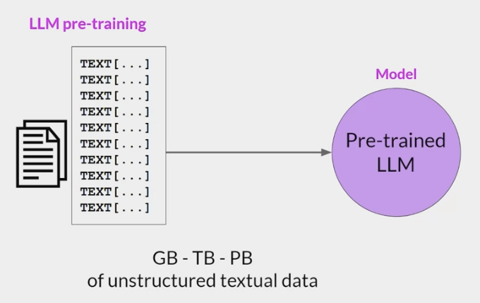
LLM - Data Tuning
LLM - Data Tuning 微调
Table of contents:
- LLM - Data Tuning 微调
- Instruction-Tuning (指示微调)
- Fine-Tuning (微调)
- LLM Evaluation
- Adapt and align large language models
- Traning Terms
ref:
- https://gitcode.csdn.net/65e93d1e1a836825ed78e986.html
overview
目前学术界一般将 NLP 任务的发展分为四个阶段,即 NLP 四范式: [^通俗易懂的LLM(上篇)]
- 第一范式: 基于「
传统机器学习模型」的范式,如 TF-IDF 特征+朴素贝叶斯等机器算法; 第二范式: 基于「
深度学习模型」的范式,如 word2vec 特征+LSTM 等深度学习算法,相比于第一范式,模型准确有所提高,特征工程的工作也有所减少;第三范式: 基于「
预训练模型+fine-tuning」的范式,如 Bert+fine-tuning 的 NLP 任务,相比于第二范式,模型准确度显著提高,模型也随之变得更大,但小数据集就可训练出好模型;- 第四范式: 基于「
预训练模型+Prompt+预测」的范式,如 Bert+Prompt 的范式相比于第三范式,模型训练所需的训练数据显著减少。
在整个 NLP 领域,你会发现整个发展是朝着精度更高 少监督,甚至无监督的方向发展的。下面我们对第三范式 第四范式进行详细介绍。
- 总的来说
- 基于 Fine-Tuning 的方法是让预训练模型去迁就下游任务。
- 基于 Prompt-Tuning 的方法可以让下游任务去迁就预训练模型。
LLM 模型训练过程中的三个核心步骤
- 预训练语言模型 $LLM^{SSL}$ (self-supervised-learning)
- (指令)监督微调预训练模型 $LLM^{SFT}$ (supervised-fine-tuning)
- 基于人类反馈的强化学习微调 $LLM^{RL}$ (reinforcement-learning)
Summary:
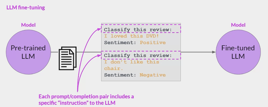
- Instruction fine-tuning updates model weights using labeled datasets, whereas in-context learning uses examples during inference.
- Prompt tuning adjusts only a few parameters (tokens), not all hyperparameters of the model.
- Catastrophic forgetting occurs when fine-tuning on a single task degrades performance on other tasks.
- BLEU (Bilingual Evaluation Understudy) measures precision by comparing generated text to reference translations.
- FLAN-T5 used multi-task finetuning, which helps prevent catastrophic forgetting.
- Smaller LLMs struggle with few-shot learning as they have limited capacity to generalize from small examples.
- Reparameterization and Additive are two PEFT methods that adjust or add parameters to efficiently fine-tune models.
- PEFT methods like LoRA can dramatically reduce memory needed for fine-tuning.
LoRA (Low-Rank Adaptation) optimizes by focusing on smaller matrices, reducing the computational load. it decomposes weights into two smaller rank matrices and trains those instead of the full model weights.
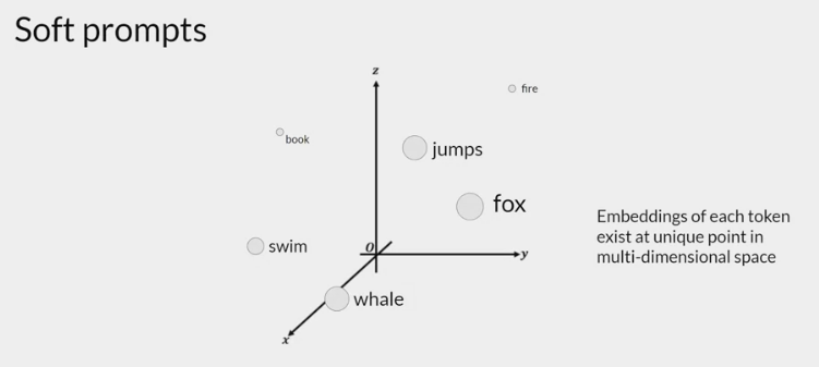
Soft prompts are trainable tokens used to guide the model’s performance on specific tasks. A set of trainable tokens that are added to a prompt and whose values are updated during additional training to improve performance on specific tasks.
- to prevent catastrophic forgetting it is important to fine-tune on multiple tasks with a lot of data.
改進 LLM
怎麼使用、使用哪個 LLM 來部屬產品? [^如何改進LLM]
- 用 GPT4 還是 GTP3.5?Llama 聽說不錯?
- 用 API 來服務還是要自己訓練、部屬模型?
- 需要 Finetune 嗎?
- 要做 prompt engineering 嗎?怎麼做?
- 要做 retrieval 嗎?,RAG(Retrieval Augmented Generation)架構對我的任務有幫助嗎?
- 主流模型就有十多個、Training 有數十種的方法,到底該怎麼辦?
- ……
FSDL 的課程:
- 李宏毅老師
- Deep Learning.ai 的 Andrew Ng 老師
- UCBerkeley 的 Full Stack Deep Learning
要選擇各種 ML DL 的技巧之前,先分清楚遇到的問題 + 哪些方法可以解決這個問題
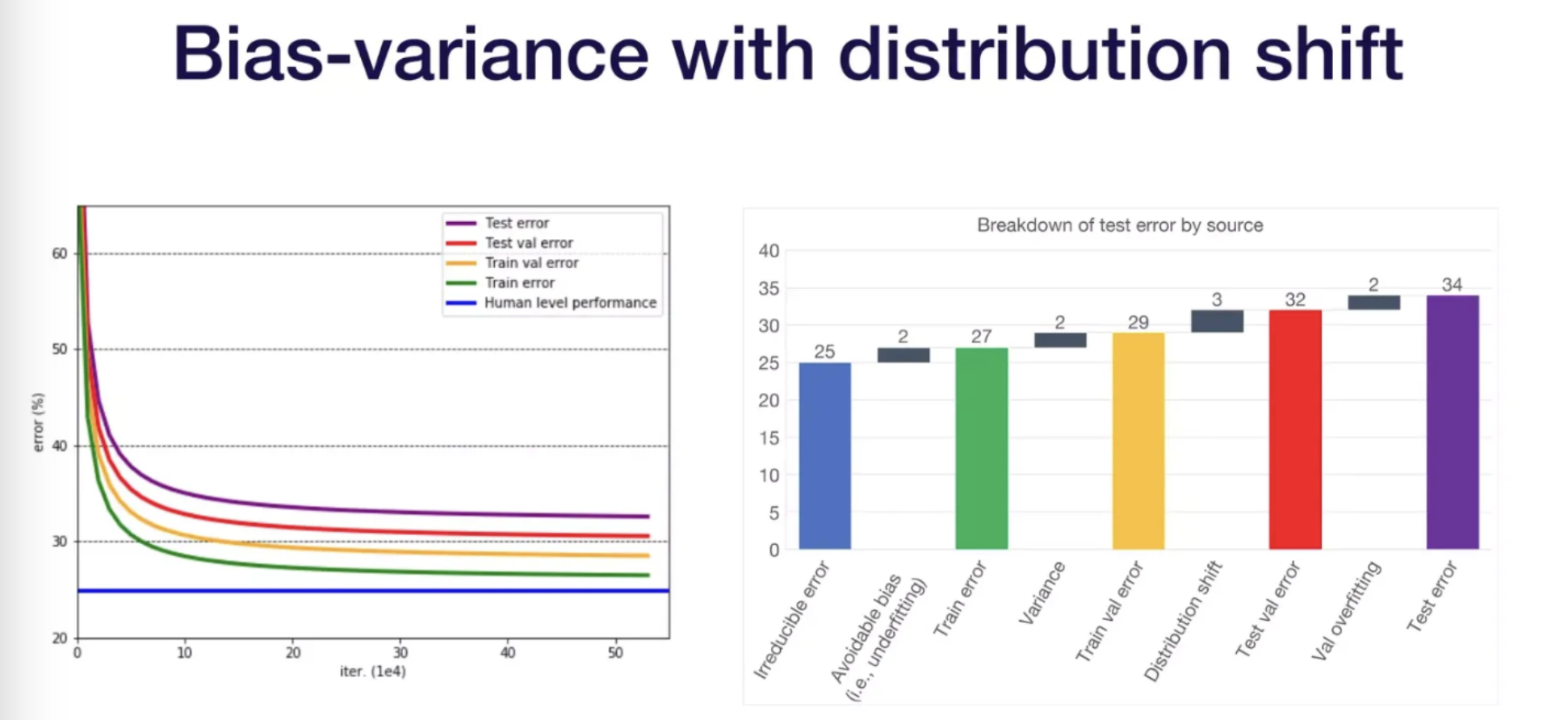
- 如果 Training Error 比 Testing Error 低一截,那我們遇到的就是
Overfitting,各種類型的 regularization 或是縮小 model 都可以派上用場。 - 但是如果我們遇到的是 Training Error 跟 Human 的水平有一截差距,那變成我們是
Underfitting,反而是要加大 model 甚至是重新定義問題,找到一個更好 fit 的問題。
從能找到的最強 LLM(GPT4)開始
- 從手邊能找到的最強 LLM 開始產品
- 對於任何一個 AI 產品而言,同時要面對兩個不確定性:1. 需求的不確定,2. 技術的不確定 。
- 技術的不確定指的是: 我們沒辦法在訓練模型之前知道我們最後可以得到的 Performance 。因此很多 AI 產品投入了資源收集資料及訓練模型,最後卻發現模型遠沒有達到可接受的標準。
在 LLM 時期其實像是 GPT4 或是 Bard 這種模型,反倒提供給我們一個非常強的 Baseline,所以先使用能找到的最強模型來開始產品。
- 先用 GPT4 來做 MVP ,如果可行則確認 unit economics、尋找護城河跟盡量減低 cost。
- 分析錯誤來源
- 如果錯誤跟 factual 比較有關, 藉由跑「給定相關資訊來進行預測」的實驗測試 LLM 到底是不具備相關知識還是 Hallucination 。
- 如果錯誤跟 reasoning 比較有關,藉由 perplexity 區分 model 需要 language modeling finetuning 還是 supervised finetuning。
- 如果 finetuning 是可行的(有一定量資料、成本可接受),直接跑小範圍的 finetune 可以驗證很多事情。
如果 LLM 沒有達成標準
如果達成標準, 則思考更多商業上的問題
確認 unit economics :
- 確保每一次用戶使用服務時,你不會虧錢。
- Ex:用戶訂閱你服務一個月只要 120,但是他平均每個月會使用超過 120 元的 GPT-4 額度,這就會出現問題(除非你有更完備的商業規劃)。
找尋護城河 :
- 因為你目前是使用第三方提供的 LLM,所以你技術上不具備獨創性,請從其他方面尋找護城河。
在達成標準的前提下盡量降低 cost :
- 換小模型
- 在傳統 chatbot 中大多有一個功能是開發者提供 QA pairs,然後每次用戶問問題,就從這些 QA pairs 中找尋最佳的回答,而 GPT cache 其實就是把每次 GPT 的回答記起來,當成一個 QA pair,新問題進來時就可以先找有沒有相似的問題,減少訪問 GPT API 的次數。
- 限縮 LLM 使用場景。
如果 LLM 沒有達成標準
如果沒有達成標準,則需要思考技術上的改進策略。分析 LLM 失敗的原因。
通常來說,LLM 會失敗主流會有 4 種原因,兩種大的類別:
- Factual 事實相關
- Reasoning 推理相關
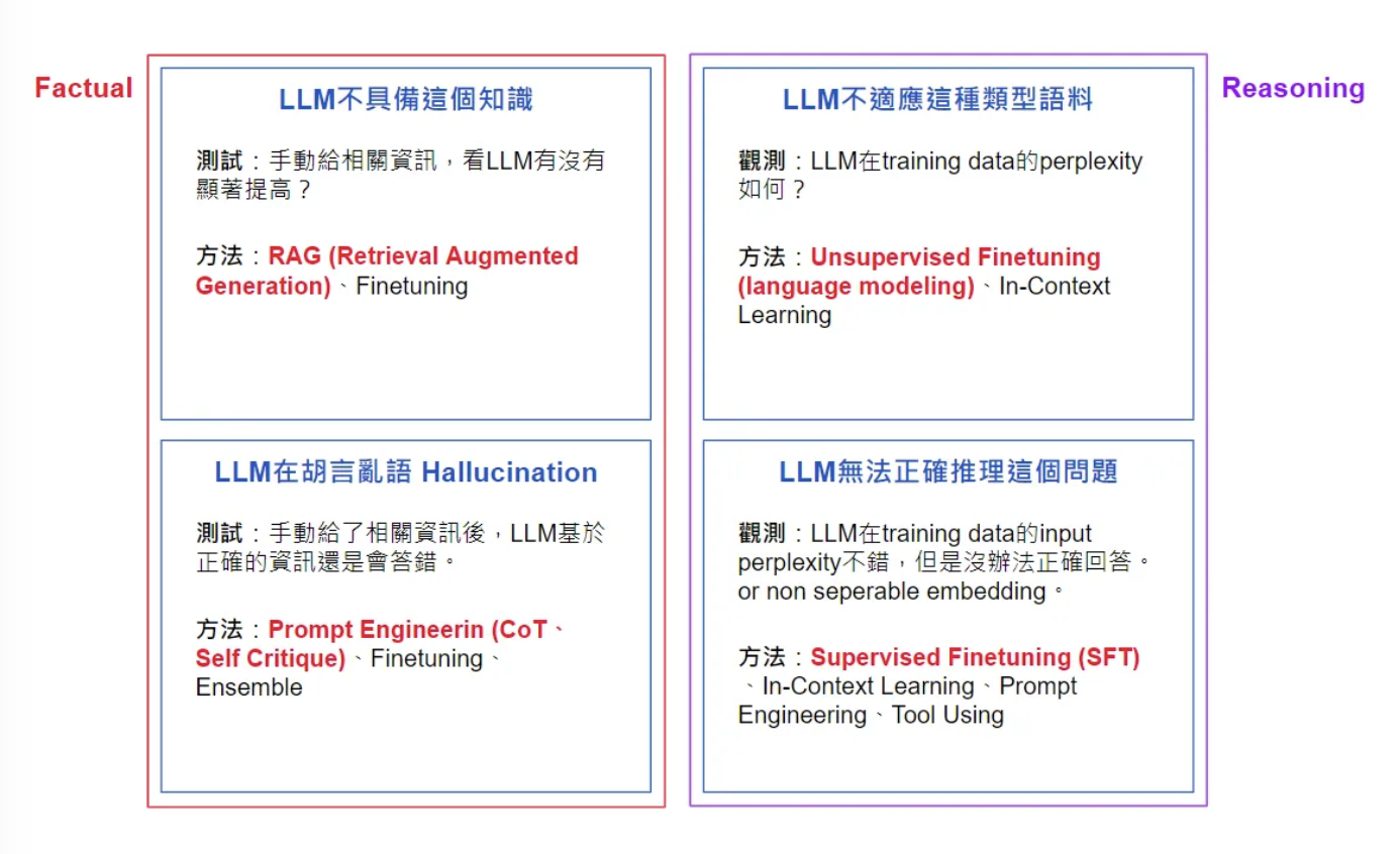
(Factual 相關)LLM 不具備這個知識 :
- 嘗試 RAG(Retrieval Augmented Generation)
- finetuning
(Factual 相關)LLM 在胡言亂語(Hallucination) :
- prompt engineering (CoT, Self Critique),
- finetuning
(Reasoning 相關)LLM 不適應這種類型語料 :
- finetuning: language modeling,
- 更換 LLM
(Reasoning 相關)LLM 無法正確推理這個問題 :
- finetuning: supervised finetuning,
- In-Context Learning
Factual 相關
- 如果 LLM 回答問題錯誤,
- 有可能是 LLM 根本不具備相關知識,導致他只能隨便回答,
- 也有可能試產生了 Hallucination(胡言亂語)的現象
而最好區分這兩者的方法,就是做以下實驗。
ICL + Retrieval Augmented Generation
- 選定 k 筆 LLM 答錯的資料
- 在 prompt 中加入能夠回答這題的相關資訊(也是你確定你未來可以取得的相關資訊),檢測是否有 明顯變好
- 如果有的話那就可以走 RAG(Retrieval Augmented Generation) 這條路
- 如果還是有一定比例的資料無法達成,那則加入像是 self critique 之類的 prompt engineering 的方法。
更直覺的思考方式:
- 你想要 LLM 完成的這個任務,會不會在網路上常常出現?
- 如果會常常出現,那高機率用 Prompt engineering 就可以,
- 如果是冷門資訊,甚至是網路上不會出現的資訊(機構內部資訊),那就一定要走 RAG。
- Ex:
- 開發銀行的客服機器人->RAG
- 開發一個每天誇獎對話機器人,高機率只要 prompr engineering,因為誇獎的用詞、知識、方法網路上出現很多次。
Reasoning 相關
- 如果 LLM 有相關知識,但是回答的時候錯誤率依舊很高,那就要考慮是不是 LLM 根本 不具備需要的推理能力 。
- 而這又分為兩種:
- LLM 對這種類型的文本不熟悉,
- LLM 對這種類型的推理、分類問題不熟悉。
- 兩者最直接的區分方法: 讓 LLM 在你對應的文本算 perplexity。
perplexity 是用來衡量「LLM 預測下一個詞的混亂程度」
如果 perplexity 高
- 代表 LLM 對這類型的文本領域(domain)根本不熟,可能是語言不熟悉,也有可能是內容領域不熟悉
- 這時候就一定要
language model finetuning,藉由unsupervised finetuning,加強 LLM 對文本領域的熟悉度。
如果 perplexity 很低,但是問題還是解決不好
- 則更需要訓練 LLM 處理特定的問題,因此則要
supervised finetuning,這就類似傳統finetune CNN,蒐集Label data,讓模型學會執行對應任務。
- 則更需要訓練 LLM 處理特定的問題,因此則要
如果是利用 GPT4 之類的 API,沒辦法取得 perplexity 的數值
- 可以從文本中找出你認為基礎的知識語句,找個 100 句,每一句拋棄後半段請 GPT4 自行接龍,再基於結果判斷 LLM 到底有沒有你這個領域的經驗。
perplexity 是高是低,其實是一個非常需要經驗的事情,所以只能當作參考指標。
- 如果一個 model 對文本的
embedding你可以取得,那可以對 embedding 去train linear classifier - 如果 non separable,則表示這個 model 無法足夠細緻的處理這類型的問題,則更需要 supervised finetuning。
- 如果一個 model 對文本的
只要 finetuning 對你而言是可以承擔的事情
- 建議對任何任務都先跑 100~1,000 筆資料、1 個 epoch 的 supervised finetuning,和 10,000 個 token 的 language modeling
- 這會更像是以前 DL 我們直接用訓練來觀測模型是否會有顯著改善。
Instruction-Tuning (指示微调)
目前最火的研究范式,性能超过包括 ICL 在内的 prompt learning
一种特别适合改进模型在多种任务上表现的策略
提出的动机:
大规模的语言模型 如 GPT-3 在 zero-shot 上不那么成功, 但却可以非常好地学习 few-shot
一些模型能够识别提示中包含的指令并正确进行 zero-shot 推理,而较小的 LLM 可能在执行任务时失败,
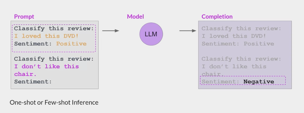
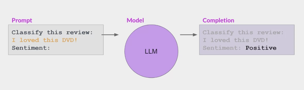
包含一个或多个你希望模型执行的示例(称为一次或几次推理)足以帮助模型识别任务并生成良好的完成结果。
然而缺点有:
对于较小的模型,即使包含 5-6 个示例,也不总是有效
提示中包含的任何示例都会占据上下文窗口中宝贵的空间,从而减少包含其他有用信息的空间
例如: GPT-3 在阅读理解 问题回答和自然语言推理等任务上的表现很一般
Google2021 年的 FLAN 模型《FINETUNED LANGUAGE MODELS ARE ZERO-SHOT LEARNERS》,这篇文章明确提出 Instruction-Tuning(指令微调)的技术,
本质目的:
- 将 NLP 任务转换为自然语言指令,再将其投入模型进行训练
- 通过给模型提供指令和选项的方式,使其能够提升 Zero-Shot 任务的性能表现。
作者认为一个潜在的原因是,如果在没有少量示例的 zero-shot 条件下,模型很难在 prompts 上表现很好,因为 prompts 可能和预训练数据的格式相差很大。
- 既然如此,那么为什么不直接用自然语言指令做输入呢?
通过设计 instruction,让大规模语言模型理解指令,进而完成任务目标,而不是直接依据演示实例做文本生成。
如下图所示,不管是 commonsense reasoning 任务还是 machine translation 任务,都可以变为 instruction 的形式,然后利用大模型进行学习。
在这种方式下,当一个 unseen task 进入时,通过理解其自然语言语义可以轻松实现 zero-shot 的扩展,如 natural language inference 任务。
Instruction-Tuning 也是 ICL 的一种,只是 Instruction-Tuning 是将大模型在多种任务上进行微调,提升大模型的自然语言理解能力,最终实现在新任务上的 zero-shot
这些提示完成示例允许模型学习生成遵循
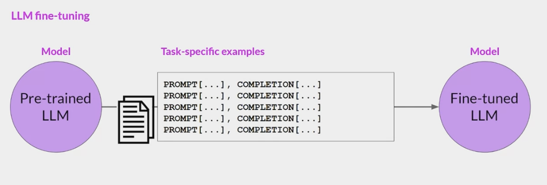
给定指令的响应。所有模型权重都会更新的指令微调过程称为全微调- 该过程生成了一个具有更新权重的模型的新版本
- 需要注意的是,与预训练一样,全微调需要足够的内存和计算预算来存储和处理所有梯度、优化器和其他在训练过程中被更新的组件


采用了 Instruction-Tuning 技术的大规模语言模型
- instructGPT
- Finetuned Language Net(FLAN)
Finetuned Language Net(FLAN) 的具体训练流程:
- FLAN 模型将 62 个 NLP 任务分为 12 个簇,同一个簇内是相同的任务类型

对于每个 task,将为其手动构建 10 个独特 template,作为以自然语言描述该任务的 instructions。
- 为了增加多样性,对于每个数据集,还包括最多三个“turned the task around/变更任务”的模板(例如,对于情感分类,要求其生成电影评论的模板)。
- 所有数据集的混合将用于后续预训练语言模型做 Instruction-Tuning,其中每个数据集的 template 都是随机选取的。
- 如下图所示,Premise Hypothesis Options 会被填充到不同的 template 中作为训练数据。

- 最后基于 LaMDA-PT 模型进行微调。
- LaMDA-PT 是一个包含 137B 参数的自回归语言模型,这个模型在 web 文档(包括代码) 对话数据和维基百科上进行了预训练,同时有大约 10%的数据是非英语数据。然后 FLAN 混合了所有构造的数据集在 128 核的 TPUv3 芯片上微调了 60 个小时。
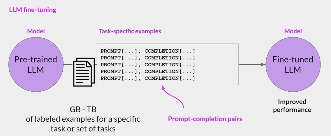
Fine-Tuning (微调)
Fine-Tuning 是一种迁移学习,在自然语言处理(NLP)中,Fine-Tuning 是用于将预训练的语言模型适应于特定任务或领域。
基本思想是采用已经在大量文本上进行训练的预训练语言模型,然后在小规模的任务特定文本上继续训练它。
Fine-Tuning 的概念已经存在很多年,并在各种背景下被使用。
- Fine-Tuning 在 NLP 中最早的已知应用是在神经机器翻译(NMT)的背景下,其中研究人员使用预训练的神经网络来初始化一个更小的网络的权重,然后对其进行了特定的翻译任务的微调。
经典的 Fine-Tuning 方法包括将预训练模型与少量特定任务数据一起继续训练。
- 在这个过程中,预训练模型的权重被更新,以更好地适应任务。
- 所需的 Fine-Tuning 量取决于预训练语料库和任务特定语料库之间的相似性。
- 如果两者相似,可能只需要少量的 Fine-Tuning,如果两者不相似,则可能需要更多的 Fine-Tuning。
Bert 模型 2018 年横空出世之后,将 Fine-Tuning 推向了新的高度。不过目前来看,Fine-Tuning 逐渐退出了 tuning 研究的舞台中心: LLM 蓬勃发展,Fine-Tuning 这种大规模更新参数的范式属实无法站稳脚跟。而更适应于 LLM 的 tuning 范式,便是接下来我们要介绍的 Prompt-Tuning Instruction-Tuning 等。
Full Fine-tuning
Self-supervised-learning 预训练阶段
- 从互联网上收集海量的文本数据,通过自监督的方式训练语言模型,根据上下文来预测下个词。
- token 的规模大概在 trillion 级别,这个阶段要消耗很多资源,海量的数据采集 清洗和计算,
- 该阶段的目的是:通过海量的数据,让模型接触不同的语言模式,让模型拥有理解和生成上下文连贯的自然语言的能力。

训练过程大致如下:
| name | des |
|---|---|
| Training data | 来自互联网的开放文本数据,整体质量偏低 |
| Data scale | 词汇表中的 token 数量在 trillion 级别 |
| $LLM^{SSL}_ϕ$ | 预训练模型 |
| $V$ | 词汇表的大小 |
| $[T_1,T_2,…,T_V]$ | vocabulary 词汇表,训练数据中词汇的集合 |
| $f(x)$ | 映射函数把词映射为词汇表中的索引即:token. |
| . | if $x$ is $T_k$ in vocab, $f(x) = k$ |
| $(x_1,x_2,…,x_n)$ | 根据文本序列生成训练样本数据: |
| . | Input: $x=(x_1,x_2,…,x_{i−1})$ |
| . | Output(label) : $x_i$ |
| $(x,xi)$ | 训练样本: |
| . | Let $k = f(x_i), word→token$ |
| . | Model’s output: $LLM^{SSL}(x)=[\bar{y_1},\bar{y2},…,\bar{yV}]$ |
| . | 模型预测下一个词的概率分布,Note : $∑_j \bar{y_j} = 1$ |
| . | The loss value:$CE(x,x_i;ϕ)= −log(\overline{y}_k)$ |
Goal : find $ϕ$, Minimize $CE(\phi) = -E_x log(\overline{y}_k)$
预先训练阶段 $LLM^{SSL}$ 还不能正确的响应用户的提示
- 例如,如果提示“法国的首都是什么?”这样的问题,模型可能会回答另一个问题的答案,例如,模型响应的可能是“意大利的首都是什么?”
- 因为模型可能没有“理解”/“对齐 aligned”用户的“意图”,只是复制了从训练数据中观察到的结果。
为了解决这个问题,出现了一种称为监督微调或者也叫做指令微调的方法。
- 通过在少量的示例数据集上采用监督学习的方式对 $LLM^{SSL}$ 进行微调,经过微调后的模型,可以更好地理解和响应自然语言给出的指令。
SFT - Supervised Fine-Tuning (监督微调阶段)
Overview
good option when you have a well-defined task with available labeled data.
particularly effective for domain-specific applications where the language or content significantly differs from the data the large model was originally trained on.
Supervised fine-tuning adapts model behavior with a labeled dataset.
- This process adjusts the model’s weights to
minimize the difference between its predictions and the actual labels.
For example, it can improve model performance for the following types of tasks:
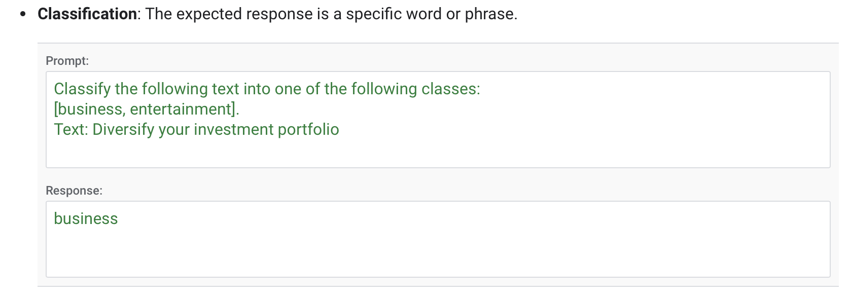
- Classification
- Summarization
- Extractive question answering
- Chat

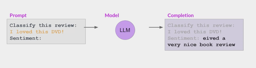
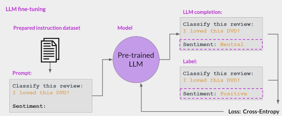
SFT(Supervised Fine-Tuning)阶段的目标是
优化预训练模型,使模型生成用户想要的结果。- 在该阶段,给模型展示
如何适当地响应不同的提示 (指令) (例如问答,摘要,翻译等)的示例。 - 这些示例遵循 (prompt response)的格式,称为演示数据。
- 通过基于示例数据的监督微调后,模型会模仿示例数据中的响应行为,学会问答 翻译 摘要等能力,
- OpenAI 称为:监督微调行为克隆 。
- 在该阶段,给模型展示
- 基于 LLM 指令微调的突出优势在于,对于任何特定任务的专用模型,只需要在通用大模型的基础上通过特定任务的指令数据进行微调,就可以解锁 LLM 在特定任务上的能力
- 不需要从头去构建专用的小模型。
- 事实也证明,经过微调后的小模型可以生成比没有经过微调的大模型更好的结果:
指令微调过程如下:
1
2
3
4
5
6
7
8
9
10
11
12
13
- Training Data : 高质量的微调数据,由人工产生。

- Data Scale : 10000~100000

  - InstructGPT : ~14500 个人工示例数据集。
  - Alpaca : 52K ChatGPT 指令数据集。

- Model input and output

  - Input : 提示 (指令)。
  - Output : 提示对应的答案(响应)

- Goal : 最小化交叉熵损失,只计算出现在响应中的 token 的损失。
Implementation in GCP
Recommended configurations
- The following table shows the recommended configurations for tuning a foundation model by task:
| Task | No. of examples in dataset | Number of epochs |
|---|---|---|
| Classification | 500+ | 2-4 |
| Summarization | 1000+ | 2-4 |
| Extractive QA | 500+ | 2-4 |
| Chat | 1000+ | 2-4 |
- import lib
1
2
3
4
5
6
7
8
9
10
11
12
13
14
15
16
17
18
19
20
21
22
23
24
25
26
27
28
import time
from typing import Dict, List

# For data handling.
import pandas as pd

# For visualization.
import plotly.graph_objects as go

# For fine tuning Gemini model.
import vertexai

# For extracting vertex experiment details.
from google.cloud import aiplatform
from google.cloud.aiplatform.metadata import context
from google.cloud.aiplatform.metadata import utils as metadata_utils
from plotly.subplots import make_subplots

# For evaluation metric computation.
from rouge_score import rouge_scorer
from tqdm import tqdm
from vertexai.generative_models import (
    GenerationConfig,
    GenerativeModel,
    HarmBlockThreshold,
    HarmCategory,
)
from vertexai.preview.tuning import sft
- setup env
1
2
3
PROJECT_ID = "the_id"  # @param
LOCATION = "us-central1"  # @param
vertexai.init(project=PROJECT_ID, location=LOCATION)
- Dataset
1
2
3
4
5
6
7
8
9
10
11
12
13
14
15
16
17
18
19
20
21
22
23
24
25
26
27
28
29
30
31
32
33
34
35
36
37
38
39
40
41
42
43
44
45
46
47
48
49
# ++++++++ Dataset Citation ++++++++
@inproceedings{
    ladhak-wiki-2020,
    title={WikiLingua: A New Benchmark Dataset for Multilingual Abstractive Summarization},
    author={Faisal Ladhak, Esin Durmus, Claire Cardie and Kathleen McKeown},
    booktitle={Findings of EMNLP, 2020},
    year={2020}
}

# Dataset for model tuning.
training_data_path = "gs://github-repo/generative-ai/gemini/tuning/summarization/wikilingua/sft_train_samples.jsonl"
# Dataset for model evaluation.
validation_data_path = "gs://github-repo/generative-ai/gemini/tuning/summarization/wikilingua/sft_val_samples.jsonl"
# Dataset for model testing.
testing_data_path = "gs://github-repo/generative-ai/gemini/tuning/summarization/wikilingua/sft_test_samples.csv"

# Provide a bucket name
BUCKET_NAME = "the_bucket_id"  # @param {type:"string"}
BUCKET_URI = f"gs://{BUCKET_NAME}"
# Copy the tuning and evaluation data to the bucket.
!gsutil cp $training_data_path {BUCKET_URI}/sft_train_samples.jsonl
!gsutil cp $validation_data_path {BUCKET_URI}/sft_val_samples.jsonl


# ++++++++ Test dataset ++++++++
# Load the test dataset using pandas as it's in the csv format.
test_data = pd.read_csv(testing_data_path)
test_data.head()
test_data.loc[0, "input_text"]

# Article summary stats
stats = test_data["output_text"].apply(len).describe()
stats

print(f"Total `{stats['count']}` test records")
print(f"Average length is `{stats['mean']}`")
print(f"Max is `{stats['max']}` characters")

# Get ceil value of the tokens required.
print("Considering 1 token = 4 chars")
tokens = (stats["max"] / 4).__ceil__()
print(
    f"Set max_token_length = stats['max']/4 = {stats['max']/4} ~ {tokens} characters"
)
print(f"Let's keep output tokens up to `{tokens}`")

# Maximum number of tokens that can be generated in the response by the LLM.
# Experiment with this number to get optimal output.
max_output_tokens = tokens
- Test Pre-performance
1
2
3
4
5
6
7
8
9
10
11
12
13
14
15
16
17
18
19
test_doc = test_data.loc[0, "input_text"]

prompt = f"""
Article: {test_doc}
"""

generation_model = GenerativeModel("gemini-1.0-pro-002")
generation_config = GenerationConfig(
    temperature=0.1,
    max_output_tokens=max_output_tokens,
)
response = generation_model.generate_content(
    contents=prompt,
    generation_config=generation_config
).text
print(response)

# Ground truth
test_data.loc[0, "output_text"]
- Evaluation before tuning
1
2
3
4
5
6
7
8
9
10
11
12
13
14
15
16
17
18
19
20
21
22
23
24
25
26
27
28
29
30
31
32
33
34
35
36
37
38
39
40
41
42
43
44
45
46
47
48
49
50
51
52
53
54
55
56
57
58
59
60
61
62
63
64
65
66
67
68
69
70
71
72
73
74
75
76
77
78
79
80
81
82
83
84
85
86
87
88
89
90
91
92
# Convert the pandas dataframe to records (list of dictionaries).
corpus = test_data.to_dict(orient="records")
# Check number of records.
len(corpus)
# Create rouge_scorer object for evaluation
scorer = rouge_scorer.RougeScorer(
["rouge1", "rouge2", "rougeL"],
use_stemmer=True
)
def run_evaluation(model: GenerativeModel, corpus: List[Dict]) -> pd.DataFrame:
"""Runs evaluation for the given model and data.
Args:
model: The generation model.
corpus: The test data.
Returns:
A pandas DataFrame containing the evaluation results.
"""
records = []
for item in tqdm(corpus):
document = item.get("input_text")
summary = item.get("output_text")
# Catch any exception that occur during model evaluation.
try:
response = model.generate_content(
document,
generation_config=generation_config,
safety_settings={
HarmCategory.HARM_CATEGORY_HARASSMENT: HarmBlockThreshold.BLOCK_NONE,
HarmCategory.HARM_CATEGORY_HATE_SPEECH: HarmBlockThreshold.BLOCK_NONE,
HarmCategory.HARM_CATEGORY_SEXUALLY_EXPLICIT: HarmBlockThreshold.BLOCK_NONE,
HarmCategory.HARM_CATEGORY_DANGEROUS_CONTENT: HarmBlockThreshold.BLOCK_NONE,
},
)
# Check if response is generated by the model, if response is empty then continue to next item.
if not (
response
and response.candidates
and response.candidates[0].content.parts
):
print(
f"Model has blocked the response for the document.\n Response: {response}\n Document: {document}"
)
continue
# Calculates the ROUGE score for a given reference and generated summary.
scores = scorer.score(target=summary, prediction=response.text)
# Append the results to the records list
records.append(
{
"document": document,
"summary": summary,
"generated_summary": response.text,
"scores": scores,
"rouge1_precision": scores.get("rouge1").precision,
"rouge1_recall": scores.get("rouge1").recall,
"rouge1_fmeasure": scores.get("rouge1").fmeasure,
"rouge2_precision": scores.get("rouge2").precision,
"rouge2_recall": scores.get("rouge2").recall,
"rouge2_fmeasure": scores.get("rouge2").fmeasure,
"rougeL_precision": scores.get("rougeL").precision,
"rougeL_recall": scores.get("rougeL").recall,
"rougeL_fmeasure": scores.get("rougeL").fmeasure,
}
)
except AttributeError as attr_err:
print("Attribute Error:", attr_err)
continue
except Exception as err:
print("Error:", err)
continue
return pd.DataFrame(records)
# Batch of test data.
corpus_batch = corpus[:100]
# Run evaluation using loaded model and test data corpus
evaluation_df = run_evaluation(generation_model, corpus_batch)
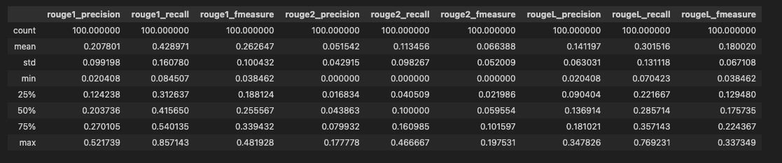
evaluation_df.head()
# Statistics of the evaluation dataframe.
evaluation_df_stats = evaluation_df.dropna().describe()
evaluation_df_stats
print("Mean rougeL_precision is", evaluation_df_stats.rougeL_precision["mean"])
| count | document | summary | generated_summary | scores | rouge1_precision | rouge1_recall | rouge1_fmeasure | rouge2_precision | rouge2_recall | rouge2_fmeasure | rougeL_precision | rougeL_recall | rougeL_fmeasure |
|---|---|---|---|---|---|---|---|---|---|---|---|---|---|
| 0 | Hold the arm out flat in front of you with yo… | Squeeze a line of lotion onto the tops of both… | This article provides instructions on how to a… | {‘rouge1’: (0.29508196721311475, 0.58064516129… | 0.295082 | 0.580645 | 0.391304 | 0.133333 | 0.266667 | 0.177778 | 0.213115 | 0.419355 | 0.282609 |
| 1 | As you continue playing, surviving becomes pai… | Make a Crock Pot for better food. Create an Al… | This article provides a guide on how to surviv… | {‘rouge1’: (0.14814814814814814, 0.66666666666… | 0.148148 | 0.666667 | 0.242424 | 0.062500 | 0.294118 | 0.103093 | 0.123457 | 0.555556 | 0.202020 |
Fine-tune the Model
source_model: Specifies the base model version you want to fine-tune.train_dataset: Path to the training data in JSONL format.- Optional parameters
validation_dataset: If provided, this data is used to evaluate the model during tuning.epochs: The number of training epochs to run.learning_rate_multiplier: A value to scale the learning rate during training.
1
2
3
4
5
6
7
8
9
10
11
12
13
14
15
16
17
18
19
20
21
22
23
24
25
26
27
28
29
# Tune a model using `train` method.
sft_tuning_job = sft.train(
    source_model="gemini-1.0-pro-002",
    train_dataset=f"{BUCKET_URI}/sft_train_samples.jsonl",
    # Optional:
    validation_dataset=f"{BUCKET_URI}/sft_val_samples.jsonl",
    epochs=3,
    learning_rate_multiplier=1,
)

# Get the tuning job info.
sft_tuning_job.to_dict()

# Get the resource name of the tuning job
sft_tuning_job_name = sft_tuning_job.resource_name
sft_tuning_job_name

%%time
# Wait for job completion
while not sft_tuning_job.refresh().has_ended:
    time.sleep(60)

# tuned model name
tuned_model_name = sft_tuning_job.tuned_model_name
tuned_model_name

# tuned model endpoint name
tuned_model_endpoint_name = sft_tuning_job.tuned_model_endpoint_name
tuned_model_endpoint_name
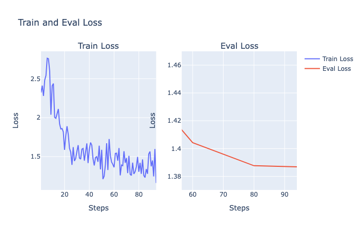
- Tuning and evaluation metrics
Model tuning metrics
/train_total_loss: Loss for the tuning dataset at a training step./train_fraction_of_correct_next_step_preds:- The token accuracy at a training step.
- A single prediction consists of a sequence of tokens.
- This metric measures the accuracy of the predicted tokens when compared to the ground truth in the tuning dataset.
/train_num_predictions: Number of predicted tokens at a training step
Model evaluation metrics:
/eval_total_loss: Loss for the evaluation dataset at an evaluation step./eval_fraction_of_correct_next_step_preds:- The token accuracy at an evaluation step.
- A single prediction consists of a sequence of tokens.
- This metric measures the accuracy of the predicted tokens when compared to the ground truth in the evaluation dataset.
/eval_num_predictions: Number of predicted tokens at an evaluation step.
The metrics visualizations are available after the model tuning job completes. If you don’t specify a validation dataset when you create the tuning job, only the visualizations for the tuning metrics are available.
1
2
3
4
5
6
7
8
9
10
11
12
13
14
15
# Get resource name from tuning job.
experiment_name = sft_tuning_job.experiment.resource_name
# Locate Vertex Experiment and Vertex Experiment Run
experiment = aiplatform.Experiment(experiment_name=experiment_name)

filter_str = metadata_utils._make_filter_string(
    schema_title="system.ExperimentRun",
    parent_contexts=[experiment.resource_name],
)
experiment_run = context.Context.list(filter_str)[0]

# Read data from Tensorboard
tensorboard_run_name = f"{experiment.get_backing_tensorboard_resource().resource_name}/experiments/{experiment.name}/runs/{experiment_run.name}"
tensorboard_run = aiplatform.TensorboardRun(tensorboard_run_name)
metrics = tensorboard_run.read_time_series_data()
- Plot the metrics
1
2
3
4
5
6
7
8
9
10
11
12
13
14
15
16
17
18
19
20
21
22
23
24
25
26
27
28
29
30
31
32
33
34
35
36
37
38
39
40
41
42
43
44
45
46
47
48
49
50
51
52
def get_metrics(metric: str = "/train_total_loss"):
    """
    Get metrics from Tensorboard.

    Args:
      metric: metric name, eg. /train_total_loss or /eval_total_loss.
    Returns:
      steps: list of steps.
      steps_loss: list of loss values.
    """
    loss_values = metrics[metric].values
    steps_loss = []
    steps = []
    for loss in loss_values:
        steps_loss.append(loss.scalar.value)
        steps.append(loss.step)
    return steps, steps_loss

# Get Train and Eval Loss
train_loss = get_metrics(metric="/train_total_loss")
eval_loss = get_metrics(metric="/eval_total_loss")

# Plot the train and eval loss metrics using Plotly python library
fig = make_subplots(
    rows=1, cols=2,
    shared_xaxes=True,
    subplot_titles=("Train Loss", "Eval Loss")
)

# Add traces
fig.add_trace(
    go.Scatter(
      x=train_loss[0], y=train_loss[1],
      name="Train Loss", mode="lines"),
    row=1, col=1,
)
fig.add_trace(
    go.Scatter(
      x=eval_loss[0], y=eval_loss[1],
      name="Eval Loss", mode="lines"),
    row=1, col=2,
)

# Add figure title
fig.update_layout(title="Train and Eval Loss", xaxis_title="Steps", yaxis_title="Loss")
# Set x-axis title
# Set y-axes titles
fig.update_xaxes(title_text="Steps")
fig.update_yaxes(title_text="Loss")

# Show plot
fig.show()
- Load the Tuned Model
1
2
3
4
5
6
7
8
if sft_tuning_job.has_succeeded:
    tuned_genai_model = GenerativeModel(tuned_model_endpoint_name)
    # Test with the loaded model.
    print("***Testing***")
    print(tuned_genai_model.generate_content(contents=prompt))
else:
    print("State:", sft_tuning_job.state)
    print("Error:", sft_tuning_job.error)
We can clearly see the difference between summary generated pre and post tuning, as tuned summary is more inline with the ground truth format (Note: Pre and Post outputs, might vary based on the set parameters.)
- Pre:
This article provides instructions on how to apply lotion to the back using the forearms. The method involves squeezing a line of lotion onto the forearms, bending the elbows, and reaching behind the back to rub the lotion on. The article also notes that this method may not be suitable for people with shoulder pain or limited flexibility. - Post:
Dispense a line of lotion onto the forearms. Place the forearms behind you. Rub the forearms up and down the back. - Ground Truth:
Squeeze a line of lotion onto the tops of both forearms and the backs of the hands. Place the arms behind the back. Move the arms in a windshield wiper motion.
- Pre:
- Evaluation post model tuning
1
2
3
4
5
6
# Run evaluation using loaded model and test data corpus
evaluation_df = run_evaluation(generation_model, corpus_batch)
evaluation_df.head()
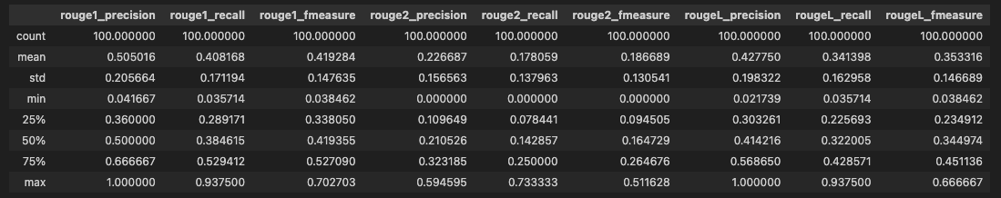
# Statistics of the evaluation dataframe.
evaluation_df_stats = evaluation_df.dropna().describe()
evaluation_df_stats
1
2
3
4
5
6
7
# run evaluation
evaluation_df_post_tuning = run_evaluation(tuned_genai_model, corpus_batch)
evaluation_df_post_tuning.head()

# Statistics of the evaluation dataframe post model tuning.
evaluation_df_post_tuning_stats = evaluation_df_post_tuning.dropna().describe()
evaluation_df_post_tuning_stats
1
2
3
4
5
6
7
8
9
10
11
print(
  "Mean rougeL_precision is",
  evaluation_df_stats.rougeL_precision["mean"]
)
# Mean rougeL_precision is 0.14326482896213358

print(
  "Mean rougeL_precision is",
  evaluation_df_post_tuning_stats.rougeL_precision["mean"]
)
# Mean rougeL_precision is 0.42774974724224635
1
2
3
4
5
6
7
8
9
10
11
12
13
14
15
improvement = round(
    (
        (
            evaluation_df_post_tuning_stats.rougeL_precision["mean"]
            - evaluation_df_stats.rougeL_precision["mean"]
        )
        / evaluation_df_stats.rougeL_precision["mean"]
    )
    * 100,
    2,
)
print(
    f"Model tuning has improved the rougeL_precision by {improvement}% (result might differ based on each tuning iteration)"
)
# Model tuning has improved the rougeL_precision by 198.57% (result might differ based on each tuning iteration)
Prompt-Oriented Fine-Tuning
需要更新全部参数(包括预训练模型参数)的 Prompt-Tuning 方法。
- 训练方法的本质是
将目标任务转换为适应预训练模型的预训练任务,以适应预训练模型的学习体系。
例如我们在 Bert 模型上做情感分类任务,
正常的 Fine-Tuning 流程,是将
训练文本经过 Bert 编码后,生成向量表征,再利用该向量表征,连接全连接层,实现最终的情感类别识别。- 这种方式存在一个显式的弊端:
预训练任务与下游任务存在gap
- 这种方式存在一个显式的弊端:
Bert 的预训练任务包括两个:
MLM与NSP(具体可参考Bert 预训练的任务 MLM 和 NSP)
MLM任务是通过分类模型识别被MASK掉的词,类别大小即为整个词表大小;NSP任务是预测两个句子之间的关系;
Prompt-Oriented Fine-Tuning 训练方法,是将情感分类任务转换为类似于
MLM任务的[Mask]预测任务:- 构建如下的 prompt 文本:
prompt = It was [MASK]. - 将 prompt 文本与输入 text 文本
text = The film is attractive.进行拼接生成It was [MASK].The film is attractive. - 输入至预训练模型中,训练任务目标和
MLM任务的目标一致,即识别被[Mask]掉的词。
- 构建如下的 prompt 文本:
通过这种方式,可以将下游任务转换为和预训练任务较为一致的任务,已有实验证明,Prompt-Oriented Fine-Tuning 相对于常规的 Fine-Tuning,效果确实会得到提升(Prompt 进行情感分类)。
- 通过以上描述我们可以知道,Prompt-Oriented Fine-Tuning 方法中,预训练模型参数是可变的。
- 其实将 Prompt-Oriented Fine-Tuning 方法放在 Prompt-Tuning 这个部分合理也不合理,因为它其实是
Prompt-Tuning+Fine-Tuning的结合体,将它视为 Fine-Tuning 的升级版是最合适的。 Prompt-Oriented Fine-Tuning 方法在 Bert 类相对较小的模型上表现较好,但是随着模型越来越大,如果每次针对下游任务,都需要更新预训练模型的参数,资源成本及时间成本都会很高,因此后续陆续提出了不更新预训练模型参数,单纯只针对 prompt 进行调优的方法,例如Hard Prompt和Soft Prompt。
- 这里再给出一些常见下游任务的 prompt 设计:

Not Full fine-tuning
XXX-of-Thoughts
CoT (Chain of Thoughts) approach
- LLMs tend to progress linearly in their thinking towards problem solving, and if an error occurs along the way, they tend to proceed along that erroneous criterion.
ToT (Tree of Thoughts) approach
- LLMs evaluate themselves at each stage of thought and stop inefficient approaches early, switching to alternative methods.
Chain-of-Thought(思维链)
随着 LLM 的越来越大,以及 tuning 技术的快速发展,LLM 在包括情感分析在内的传统自然语言任务上表现越来越好,但是单纯的扩大 LLM 模型的参数量无法让模型在算术推理/常识推理/符号推理等推理任务上取得理想的效果。 如何提升 LLM 在这些推理任务上性能呢?在此前关于 LLM 的推理任务中,有两种方法:
- 针对下游任务对模型进行微调;
- 为模型提供少量的输入输出样例进行学习。
但是这两种方法都有着局限性,前者微调计算成本太高,后者采用传统的输入输出样例在推理任务上效果很差,而且不会随着语言模型规模的增加而有实质性的改善。此时,Chain-of-Thought 应运而生。下面我们根据三篇比较有代表性的论文,详细介绍 CoT 的发展历程。
Manual-CoT(人工思维链)
Manual-CoT 是 Chain-of-Thought 技术的开山之作,由 Google 在 2022 年初提出《Chain-of-Thought Prompting Elicits Reasoning in Large Language Models》。其旨在进一步提高超大规模模型在一些复杂任务上的推理能力。其认为现有的超大规模语言模型可能存在下面潜在的问题:
- 增大模型参数规模对于一些具有挑战的任务(例如算术 常识推理和符号推理)的效果并未证明有效;
- 期望探索如何对大模型进行推理的简单方法。
针对这些问题,作者提出了 chain of thought (CoT)这种方法来利用大语言模型求解推理任务。
下面这个例子可以很好的说明思维链到底在做什么。左图是传统的 one-shot prompting,就是拼接一个例子在 query 的前面。右图则是 CoT 的改进,就是将 example 中的 Answer 部分的一系列的推理步骤(人工构建)写出来后,再给出最终答案。逻辑就是希望模型学会一步一步的输出推理步骤,然后给出结果。 
论文中首先在算数推理(arithmetic reasoning)领域做了实验,使用了 5 个数学算术推理数据集: GSM8K / SVAMP / ASDiv / AQuA / MAWPS,具体的实验过程这里不再赘述,感兴趣的同学可以直接参考论文,这里直接给出实验结论(如下图): 
- CoT 对小模型作用不大: 模型参数至少达到 10B 才有效果,达到 100B 效果才明显。并且作者发现,在较小规模的模型中产生了流畅但不符合逻辑的 CoT,导致了比 Standard prompt 更低的表现;
- CoT 对复杂的问题的性能增益更大: 例如,对于 GSM8K(baseline 性能最低的数据集),最大的 GPT (175B GPT)和 PaLM (540B PaLM)模型的性能提高了一倍以上。而对于 SingleOp(MAWPS 中最简单的子集,只需要一个步骤就可以解决),性能的提高要么是负数,要么是非常小;
- CoT 超越 SOTA: 在 175B 的 GPT 和 540B 的 PaLM 模型下,CoT 在部分数据集上超越了之前的 SOTA(之前的 SOTA 采用的是在特定任务下对模型进行微调的模式)。
除此之外,论文中为了证明 CoT 的有效性,相继做了消融实验(Ablation Study) 鲁棒性实验( Robustness of Chain of Thought) 常识推理(Commonsense Reasoning)实验 符号推理(Symbolic Reasoning)实验,下面分别做以简单介绍:
消融实验: 通过研究移除某个组件之后的性能,证明该组件的有效性。
论文中通过引入 CoT 的三个变种,证明 CoT 的有效性
结果如下图所示:

Equation only: 把 CoT 中的文字去掉,只保留公式部分。结论: 效果对于原始 prompt 略有提升,对简单任务提升较多,但和 CoT 没法比,特别是对于复杂任务,几乎没有提升。
Variable compute only: 把 CoT 中的 token 全换成点(…)。 这是为了验证额外的计算量是否是影响模型性能的因素。结论: 全换成点(…)后效果和原始 prompt 没什么区别,这说明计算量用的多了对结果影响很小(几乎没有影响),也说明了人工构建的 CoT(token sequence)对结果影响很大。
Chain of thought after answer: 把思维链放到生成结果之后。 这样做的原因是: 猜测 CoT 奏效的原因可能仅仅是这些 CoT 简单的让模型更好的访问了预训练期间获得的相关知识,而与推理没啥太大关系。结论: CoT 放到生成的答案之后的效果和 benchmark 没太大区别,说明 CoT 的顺序逻辑推理还是起到了很大作用的(不仅仅是激活知识),换句话说,模型确实是依赖于生成的思维链一步一步得到的最终结果。
鲁棒性实验: 论文中通过 annotators(标注者),exemplars(样例选择)和 models(模型)三个方面对 CoT 进行了鲁棒性分析。如下图所示,总体结论是思维链普遍有效,但是不同的 CoT 构建方式/exemplars 的选择/exemplars 的数量/exemplars 的顺序,在一定程度上影响着 CoT 的效果。

- 不同人构建 CoT: 尽管每个人构建的 CoT 都不相同,但都对模型性能产生了正面的影响,说明 CoT 确实有效。但是另一方面,不同人给出的不同的 CoT 对最终结果的影响程度还是有很大不同的,说明如何更好的构建 CoT 是一个研究方向;
- Exemplars 样本的选择: 不同的选择都会有提升,但是差异明显。特别是,在一个数据集上选择的 exemplars 可以用在其他数据集上,比如论文中的实验设置,对于同一种类型的问题,如算术推理,尽管在多个不同的数据集进行实验,但使用的是 8 个相同的 exemplars,结果没有特别大的差异,说明 exemplars 不需要满足和 test set 有相同的分布;
- Exemplars 样本的顺序: 整体影响不大,除了 coin flip task,可能的原因是: 同一个类别的多个 exemplars 连续输入模型使其输出产生了偏差(bias),例如把 4 个负样本放到 4 个正样本的后面输入到模型中,可能导致模型更加倾向于输出负 label;
- Exemplars 样本的数量: 对于标准 prompt,增加 exemplars 的数量对最终结果的影响不大。对于 CoT,增加 exemplars 对模型有影响(在某些数据集上),同时也不是越大越好;
- 不同 LLM 上的效果: 对于一个 LLM 效果好的 CoT exemplars set 换到其他 LLM 上效果不一定好,也就是说 CoT 对模型的提升是无法在不同的 LLM 上传递的,这是一个局限。
关于鲁棒性实验,论文中最后指出: Prompt Engineering仍然很重要,不同的 prompt(CoT)的设计/数量/顺序都会对模型产生不同的影响,且方差还是很大的。 因此未来的一个方向可能是探索一种能够获取稳健 CoT(Prompts)的范式。 或许可以用一个 LLM 自动生成 CoT 用于 Prompting,后面我们将介绍这种技术: Auto-CoT。
常识推理实验 & 符号推理实验: 此处我们不做过多介绍,这里给出三种推理模式的 exemplars 示例(绿色: 算数推理,橙色: 常识推理,蓝色: 符号推理),供大家参考:

这篇 CoT 开山之作首次提出思维链(CoT)的概念,思维链简单的说就是一系列中间推理步骤。这篇论文最大的贡献就是发现了在 LLM 生成推理任务的结果之前,先生成思维链,会使模型的推理性能有大幅度的提升,特别是在复杂的推理任务上,但是有个前提就是 LLM 的规模要大于 10B,否则 CoT 没用甚至起副作用。CoT 的一大好处是无需微调模型参数,仅仅是改变输入就可以改进模型的性能。随着 LLM 越来越大,高校和小企业可能无法承担训练 LLM 的成本,因此无法参与其中进行科研与实践,但 CoT 这个研究方向仍然可以做。对于 CoT 的更多细节,大家可参考《Chain-of-Thought Prompting Elicits Reasoning in Large Language Models》和思维链(Chain-of-Thought, CoT)的开山之作
Zero-shot-CoT(零示例思维链)
2022 年 6 月东京大学和谷歌共同发表了一篇论文《Large Language Models are Zero-Shot Reasoners》,这是一篇关于预训练大型语言模型(Pretrained Large Language Models, LLMs)推理能力的探究论文。
目前,LLMs 被广泛运用在很多 NLP 任务上。同时,在提供了特定任务的示例之后,LLMs 是一个非常优秀的学习者。
随着思考链的提示方式(chain of thought prompting, CoT)被提出,对 LLMs 推理能力的探究上升到一个新的高度,这种提示方式可以引导模型通过示例中一步一步的推理方式,去解决复杂的多步推理,在数学推理(arithmetic reasoning)和符号推理(symbolic reasoning)中取得了 SOTA 的成果。
作者在研究中发现,对拥有 175B 参数的 GPT-3,通过简单的添加”Let’s think step by step“,可以提升模型的 zero-shot 能力。
Zero-shot-CoT 的具体格式如下图所示,需要注意一点的是,同等条件下,Zero-shot-CoT 的性能是不及 Manual-CoT 的。

Auto-CoT(自动思维链)
传统 CoT 的一个未来研究方向: 可以用一个 LLM 自动生成 CoT 用于 Prompting
- 李沐老师团队在 2022 年 10 月发表的论文《AUTOMATIC CHAIN OF THOUGHT PROMPTING IN LARGE LANGUAGE MODELS》证明了这一技术方向的有效性,称为Auto-CoT。
目前较为流行的 CoT 方法有两种,一种是 Manual-CoT,一种是 Zero-shot-CoT,两种方式的输入格式如下图所示。
- Manual-CoT 的性能是要优于 Zero-shot-CoT 的,关键原因在于 Manual-CoT 包含一些人工设计的问题 推理步骤及答案,但是这部分要花费一定的人工成本
Auto-CoT 则解决了这一痛点,具体做法是:

- 通过多样性选取有代表性的问题;
- 对于每一个采样的问题拼接上“Let’s think step by step”(类似于 Zero-shot-CoT )输入到语言模型,让语言模型生成中间推理步骤和答案,然后把这些所有采样的问题以及语言模型生成的中间推理步骤和答案全部拼接在一起,构成少样本学习的样例,最后再拼接上需要求解的问题一起输入到语言模型中进行续写,最终模型续写出了中间的推理步骤以及答案。
Auto-CoT 是 Manual-CoT 和 Zero-shot-CoT 的结合体
- 实验证明,在十个数据集上 Auto-CoT 是可以匹配甚至超越 Manual-CoT 的性能,也就说明自动构造的 CoT 的问题 中间推理步骤和答案样例比人工设计的还要好,而且还节省了人工成本。

Tree-of-Thought (ToT)
an algorithm that combines Large Language Models (LLMs) and heuristic search, as presented in this paper by Princeton University and Google DeepMind.
It appears that this algorithm is being implemented into Gemini, a multimodal generative AI that is currently under development by Google.
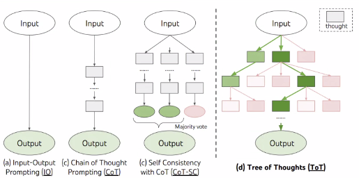
Image Source: Yao et el. (2023)
Implementation
1
2
3
4
5
6
7
8
9
10
11
12
13
14
15
16
17
18
19
20
21
22
23
24
25
26
27
28
29
30
31
32
33
34
35
36
37
38
39
40
41
42
43
44
45
46
47
48
49
50
51
52
53
54
55
56
57
58
59
60
61
62
63
64
65
66
67
68
69
70
71
72
73
74
75
76
77
78
79
80
81
82
83
84
85
86
87
88
89
90
91
92
93
94
95
from langchain.chains import LLMChain
from langchain.llms import OpenAI
from langchain.prompts import PromptTemplate
from langchain.chat_models import ChatOpenAI


template ="""
Step1 :

I have a problem related to {input}. Could you brainstorm three distinct solutions? Please consider a variety of factors such as {perfect_factors}
A:
"""

prompt = PromptTemplate(
    input_variables=["input","perfect_factors"],
    template = template
)

chain1 = LLMChain(
    llm=ChatOpenAI(temperature=0, model="gpt-4"),
    prompt=prompt,
    output_key="solutions"
)

template ="""
Step 2:

For each of the three proposed solutions, evaluate their potential. Consider their pros and cons, initial effort needed, implementation difficulty, potential challenges, and the expected outcomes. Assign a probability of success and a confidence level to each option based on these factors

{solutions}

A:"""

prompt = PromptTemplate(
    input_variables=["solutions"],
    template = template
)

chain2 = LLMChain(
    llm=ChatOpenAI(temperature=0, model="gpt-4"),
    prompt=prompt,
    output_key="review"
)

template ="""
Step 3:

For each solution, deepen the thought process. Generate potential scenarios, strategies for implementation, any necessary partnerships or resources, and how potential obstacles might be overcome. Also, consider any potential unexpected outcomes and how they might be handled.

{review}

A:"""

prompt = PromptTemplate(
    input_variables=["review"],
    template = template
)

chain3 = LLMChain(
    llm=ChatOpenAI(temperature=0, model="gpt-4"),
    prompt=prompt,
    output_key="deepen_thought_process"
)

template ="""
Step 4:

Based on the evaluations and scenarios, rank the solutions in order of promise. Provide a justification for each ranking and offer any final thoughts or considerations for each solution
{deepen_thought_process}

A:"""

prompt = PromptTemplate(
    input_variables=["deepen_thought_process"],
    template = template
)

chain4 = LLMChain(
    llm=ChatOpenAI(temperature=0, model="gpt-4"),
    prompt=prompt,
    output_key="ranked_solutions"
)

# We connect the four chains using ‘SequentialChain’. The output of one chain becomes the input to the next chain.

from langchain.chains import SequentialChain

overall_chain = SequentialChain(
    chains=[chain1, chain2, chain3, chain4],
    input_variables=["input", "perfect_factors"],
    output_variables=["ranked_solutions"],
    verbose=True
)

print(overall_chain({"input":"human colonization of Mars", "perfect_factors":"The distance between Earth and Mars is very large, making regular resupply difficult"}))
Output:
1
2
3
4
5
6
7
8
9
10
11
12
13
14
15
16
17
18
19
20
21
22
23
24
25
26
27
28
29
30
31
32
33
34
35
36
37
38
39
40
41
42
43
44
45
{
    "input": "human colonization of Mars",
    "perfect_factors": "The distance between Earth and Mars is very large, making regular resupply difficult",
    "ranked_solutions": {
        "Ranking_1": {
            "Justification": "Using In-Situ Resource Utilization is the most promising solution due to its potential to provide the necessary resources for a Mars colony and reduce the need for resupply missions from Earth. The medium initial effort, implementation difficulty, and potential challenges are outweighed by the high probability of success and 70% confidence level.",
            "In_Situ_Resource_Utilization_ISRU": {
                "Pros": "This solution could provide the necessary resources for a Mars colony and reduce the need for resupply missions from Earth.",
                "Cons": "ISRU is technically challenging and would require significant investment in research and development.",
                "Initial_Effort": "Medium. This would require the development of new technology and the establishment of infrastructure on Mars.",
                "Implementation_Difficulty": "Medium. ISRU is a complex task that requires advanced technology.",
                "Potential_Challenges": "Technical difficulties, high costs.",
                "Expected_Outcomes": "If successful, ISRU could provide a steady supply of resources for a Mars colony.",
                "Probability_of_Success": "High. ISRU is already being tested by NASA and other space agencies.",
                "Confidence_Level": "70%"
            }
        },
        "Ranking_2": {
            "Justification": "Building a self-sustaining colony is a promising solution due to its potential to make the Mars colony self-sufficient. However, the high initial effort, implementation difficulty, and potential challenges make it less promising than the first solution. The medium probability of success and 60% confidence level also contribute to its ranking.",
            "Building_a_Self_Sustaining_Colony": {
                "Pros": "This solution could make the Mars colony self-sufficient, reducing the need for resupply missions from Earth.",
                "Cons": "Building a self-sustaining colony is a complex task that requires advanced technology and a lot of resources.",
                "Initial_Effort": "High. This would require the development of new technology and the establishment of infrastructure on Mars.",
                "Implementation_Difficulty": "High. Building a self-sustaining colony is a complex task that requires advanced technology.",
                "Potential_Challenges": "Technical difficulties, high costs.",
                "Expected_Outcomes": "If successful, a self-sustaining colony could reduce the need for resupply missions from Earth.",
                "Probability_of_Success": "Medium. While there are significant challenges, there is also a lot of interest in building a self-sustaining colony on Mars.",
                "Confidence_Level": "60%"
            }
        },
        "Ranking_3": {
            "Justification": "While asteroid mining has the potential to provide a steady supply of resources for a Mars colony, the high initial effort, implementation difficulty, and potential challenges make it a less promising solution compared to others. The medium probability of success and 50% confidence level also contribute to its lower ranking.",
            "Terraforming_Mars": {
                "Pros": "This solution could make Mars more habitable for humans, reducing the need for life support systems and making the colony more self-sufficient.",
                "Cons": "Terraforming is a long-term process that could take centuries or even millennia. It would also require a massive amount of resources and energy.",
                "Initial_Effort": "Extremely High. Terraforming would require a massive amount of resources and energy.",
                "Implementation_Difficulty": "Extremely High. Terraforming is a long-term process that could take centuries or even millennia.",
                "Potential_Challenges": "Technical difficulties, high costs, time scale.",
                "Expected_Outcomes": "If successful, terraforming could make Mars more habitable for humans.",
                "Probability_of_Success": "Low. Terraforming is a theoretical concept and has never been attempted before.",
                "Confidence_Level": "20%"
            }
        }
    }
}
From the results reported in the figure below, ToT substantially outperforms the other prompting methods:
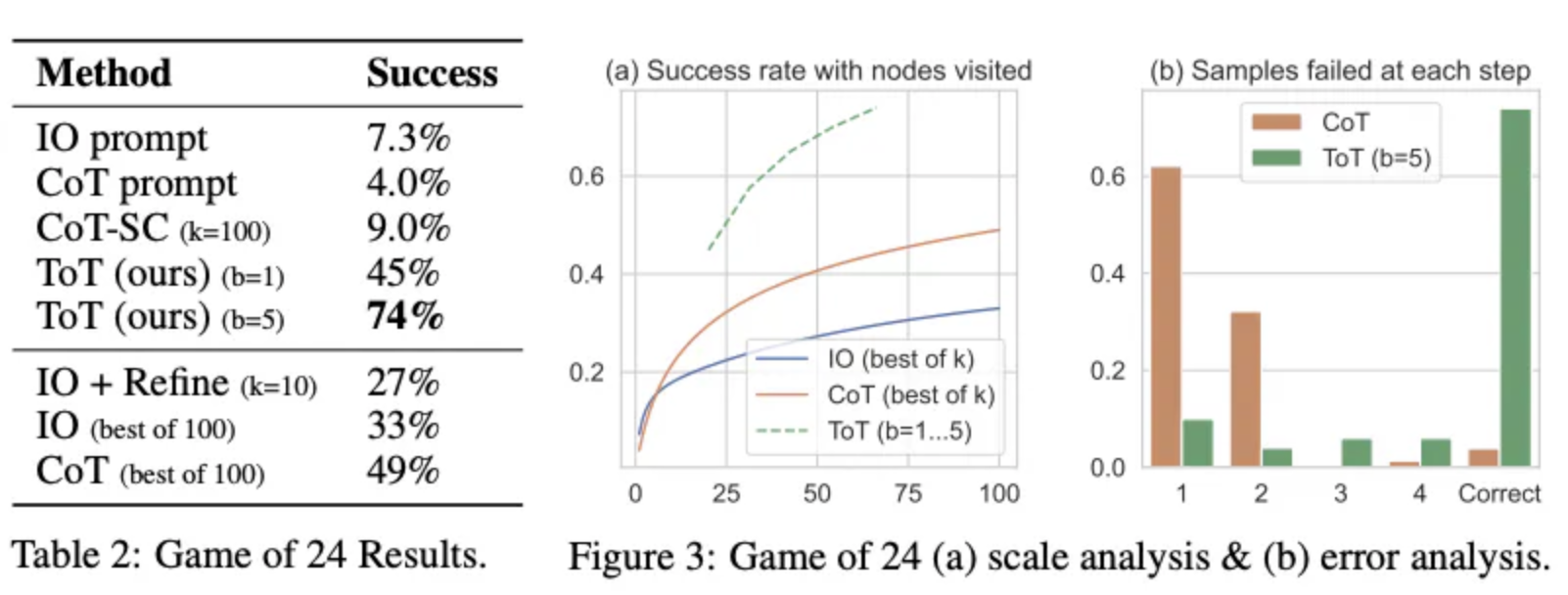
Image Source: Yao et el. (2023)
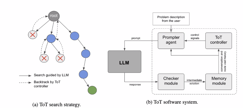
At a high level, the main ideas of Yao et el. (2023) and Long (2023) are similar.
Both enhance LLM’s capability for complex problem solving through tree search via a
multi-round conversation.One of the main difference is that Yao et el. (2023) leverages DFS/BFS/beam search, while the tree search strategy (i.e. when to backtrack and backtracking by how many levels, etc.) proposed in Long (2023) is driven by a “ToT Controller” trained through reinforcement learning.
DFS/BFS/Beam search are generic solution search strategies with no adaptation to specific problems.
In comparison, a ToT Controller trained through RL might be able learn from new data set or through self-play (AlphaGo vs brute force search), and hence the RL-based ToT system can continue to evolve and learn new knowledge even with a fixed LLM.
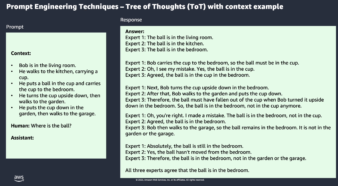
Hulbert (2023) has proposed Tree-of-Thought Prompting, which applies the main concept from ToT frameworks as a simple prompting technique, getting the LLM to evaluate intermediate thoughts in a single prompt.
- A sample ToT prompt is:
1
2
3
4
5
6
Imagine three different experts are answering this question.
All experts will write down 1 step of their thinking,
then share it with the group.
Then all experts will go on to the next step, etc.
If any expert realises they are wrong at any point then they leave.
The question is...
Sun (2023) benchmarked the Tree-of-Thought Prompting with large-scale experiments, and introduce PanelGPT — an idea of prompting with Panel discussions among LLMs.
PEFT - Parameter-Efficient Fine-Tuning (参数有效性微调)
总体来说 PEFT 可分为三个类别:
- Selective
- There are several approaches that you can take to identify which parameters you want to update.
- You have the option to train only certain components of the model or specific layers, or even individual parameter types.
- Researchers have found that the performance of these methods is mixed and there are significant trade-offs between parameter efficiency and compute efficiency
- Reparameterization
- LoRA:
- 通过学习小参数的低秩矩阵来近似模型权重矩阵的参数更新,训练时只优化低秩矩阵参数。
- LoRA:
- Additive
- keeping all of the original LLM weights frozen and introducing new trainable components.
Adapter-Tuning:
- 将较小的神经网络层或模块插入预训练模型的每一层,这些新插入的神经模块称为 adapter(适配器),下游任务微调时也只训练这些适配器参数
- add new trainable layers to the architecture of the model, typically
inside the encoder or decoder componentsafter the attention or feed-forward layers.
Soft prompt methods
- keep the model architecture fixed and frozen, and focus on manipulating the input to achieve better performance.
This can be done by adding trainable parameters to the
prompt embeddings or keeping the input fixed and retraining the embedding weights- Prompt-Tuning:
- 在模型的输入或隐层添加个额外可训练的前缀 tokens(这些前缀是连续的伪 tokens,不对应真实的 tokens),只训练这些前缀参数,包括 prefix-tuning parameter-efficient Prompt Tuning P-Tuning 等
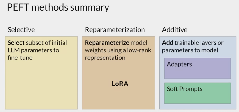
Additive
Soft prompts / Prompt-Tuning
Prompt Learning
prompt learning:
Prompt-Tuning 和 In-context learning 是 prompt learning 的两种模式。
- In-context learning
- 指在大规模预训练模型上进行推理时,不需要提前在下游目标任务上进行微调,即不改变预训练模型参数就可实现推理,
- 其认为超大规模的模型只要配合好合适的模板就可以极大化地发挥其推理和理解能力。
常用的 In-context learning 方法有
few-shot one-shot zero-shot;Prompt-Tuning
- 指在下游目标任务上进行推理前,需要对全部或者部分参数进行更新
- 全部/部分的区别就在于预训练模型参数是否改变(其实本质上的 Prompt-Tuning 是不更新预训练模型参数的,这里有个特例方法称为 Prompt-Oriented Fine-Tuning,其实该方法更适合称为升级版的 Fine-Tuning,后面会详细介绍这个方法)。
- 无论是 In-context learning 还是 Prompt-Tuning,它们的目标都是将下游任务转换为预训练模型的预训练任务,以此来广泛激发出预训练模型中的知识。
Prompting and prompt engineering:
- 如何设计输入的 prompt 是很重要的一点
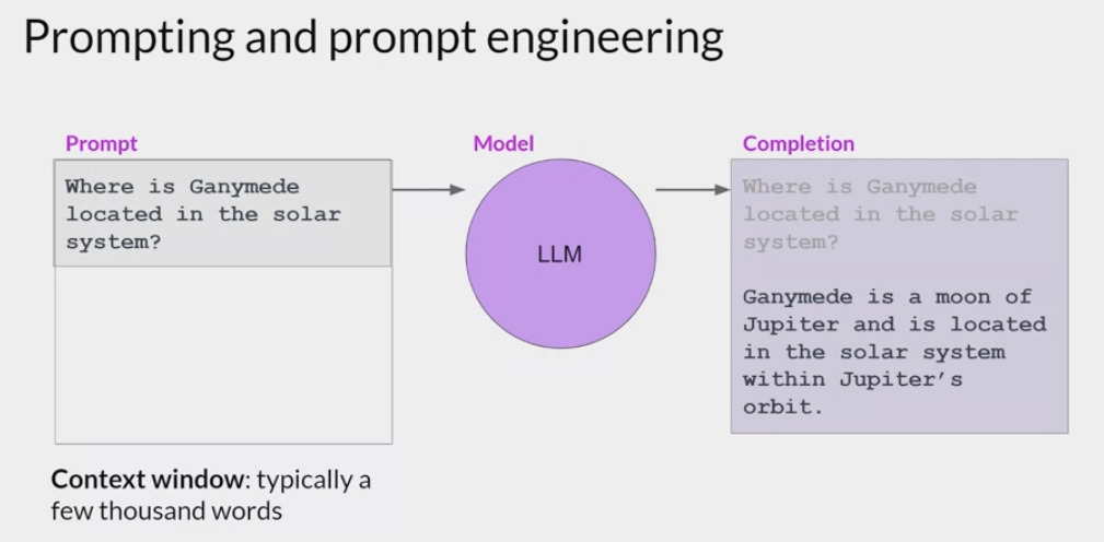
- failed with 5-6 example, fune tune the model
- Typically, above five or six shots, so full prompt and then completions, you really don’t gain much after that. Either the model can do it or it can’t do it
ICL - In-context learning (上下文学习)
- ICL 又称为上下文学习,最早是在 GPT-3《Language Models are Few-Shot Learners》中被提出来的。
ICL 的关键思想是从类比中学习。
下图给出了一个描述语言模型如何使用 ICL 进行决策的例子。
- 首先,ICL 需要一些示例来形成一个演示上下文。这些示例通常是用自然语言模板编写的。
- 然后 ICL 将查询的问题(即你需要预测标签的 input)和一个上下文演示(一些相关的 cases)连接在一起,形成带有提示的输入(可称之为 prompt),并将其输入到语言模型中进行预测。
- 值得注意的是,与需要使用反向梯度更新模型参数的训练阶段的监督学习不同,ICL 不需要参数更新,并直接对预先训练好的语言模型进行预测(这是与 Prompt-Tuning 不同的地方,ICL 不需要在下游任务中 Prompt-Tuning 或 Fine-Tuning)。
- 它希望模型能自动学习隐藏在演示中的模式,并据此做出正确的预测。

use LLMs off the shelf (i.e., without any fine-tuning), then control their behavior through clever prompting and conditioning on private “contextual” data.
it’s usually easier than the alternative: training or fine-tuning the LLM itself.
It also tends to outperform fine-tuning for relatively small datasets—since a specific piece of information needs to occur at least ~10 times in the training set before an LLM will remember it through fine-tuning—and can incorporate new data in near real time.
- Example:
- building a chatbot to answer questions about a set of legal documents.
naive approach: paste all the documents into a ChatGPT or GPT-4 prompt, then ask a question about them at the end. This may work for very small datasets, but it doesn’t scale. The biggest GPT-4 model can only process ~50 pages of input text, and performance (measured by inference time and accuracy) degrades badly when approach the limitcontext window.In-context learning: instead of sending all the documents with each LLM prompt, it sends only a handful of the most relevant documents. And the most relevant documents are determined with the help of . . . you guessed it . . . LLMs.
- building a chatbot to answer questions about a set of legal documents.
in-context learning method
One shot: creating an initial prompt that states the task to be completed and includes a single example question with answer followed by a second question to be answered by the LLM
In-context learning 的优势:
- 若干示例组成的演示是用自然语言撰写的,这提供了一个跟 LLM 交流的可解释性手段,通过这些示例跟模版让语言模型更容易利用到人类的知识;
- 类似于人类类比学习的决策过程,举一反三;
- 相比于监督学习,它不需要模型训练,减小了计算模型适配新任务的计算成本,更容易应用到更多真实场景。
In-context learning 的流程:
In-context learning 可以分为两部分,分为作用于 training 跟 inference 阶段:
Training:
在推理前,通过持续学习让语言模型的 ICL 能力得到进一步提升,这个过程称之为model warmup(模型预热),model warmup 会优化语言模型对应参数或者新增参数,区别于传统的 Fine-Tuning,Fine-Tuning 旨在提升 LLM 在特定任务上的表现,而 model warmup 则是提升模型整体的 ICL 性能。
Supervised in-context training: 为了增强 ICL 的能力,研究人员提出了
通过构建 in-context 训练数据,进而进行一系列有监督 in-context 微调以及多任务训练。由于预训练目标对于 In-context learning 并不是最优的,Sewon Min 等人提出了一种方法
MetaICL《MetaICL: Learning to Learn In Context》,以消除预训练和下游 ICL 使用之间的差距。预训练 LLM 在具有演示样例的广泛的任务上进行训练,这提高了其 few-shot 能力,例如,MetaICL获得的性能与在 52 个独力数据集上进行有监督微调相当。此外,还有一个研究方向,即有监督指令微调,也就是后面要讲到的 Instruction-Tuning。指令微调通过对任务指令进行训练增强了 LLM 的 ICL 能力。例如 Google 提出的
FLAN方法《FINETUNED LANGUAGE MODELS ARE ZERO-SHOT LEARNERS》: 通过在由自然语言指令模板构建的 60 多个 NLP 数据集上调整 137B 参数量的 LaMDA-PT 模型,FLAN 方法可以改善 zero-shot 和 few-shot ICL 性能(具体可参考Finetuned Language Models are Zero-shot Learners 笔记 - Instruction Tuning 时代的模型)。与 MetaICL 为每个任务构建若干演示样例相比,指令微调主要考虑对任务的解释,并且易于扩展。
Self-supervised in-context training:
Supervised Learning 指的是有一个 model,输入是 $x$ ,输出是 $y$ ,要有 label(标签)才可以训练 Supervised Learning,
比如让机器看一篇文章,决定文章是正面的还是负面的,得先找一大堆文章,标注文章是正面的还是负面的,正面负面就是 label。
- Self-Supervised Learning 就是机器自己在没有 label 的情况下,想办法做 Supervised Learning。
- 比如把没有标注的语料分成两部分,一部分作为模型的输入,一部分作为模型的输出,模型的输出和 label 越接近越好,具体参见2022 李宏毅机器学习深度学习学习笔记第四周–Self-Supervised Learning。
- 引申到 self-supervised in-context training,是根据 ICL 的格式将原始数据转换成 input-output 的 pair 对数据后利用四个自监督目标进行训练,包括掩
[Mask]预测,分类任务等。
Supervised ICT跟self-supervised ICT旨在通过引入更加接近于ICT的训练目标从而缩小预训练跟ICL之间的差距。- 比起需要示例的 In-context learning,只涉及任务描述的 Instruction-Tuning 更加简单且受欢迎。
- 另外,在 model warmup 这个阶段,语言模型只需要从少量数据训练就能明显提升 ICL 能力,不断增加相关数据并不能带来 ICL 能力的持续提升。
- 从某种角度上看,这些方法通过更新模型参数可以提升 ICL 能力也表明了原始的 LLM 具备这种潜力。
- 虽然 ICL 不要求 model warmup,但是一般推荐在推理前增加一个 model warmup 过程
- ICL 最初的含义指的是大规模语言模型涌现出一种能力: 不需要更新模型参数,仅仅修改输入 prompt 即添加一些例子就可以提升模型的学习能力。ICL 相比之前需要对模型在某个特定下游任务进行 Fine-Tuning 大大节省了成本。之后 ICL 问题演变成研究怎么提升模型以具备更好更通用的 ICL 能力,这里就可以用上之前 Fine-Tuning 的方式,即指 model warmup 阶段对模型更新参数
Inference:
很多研究表明 LLM 的 ICL 性能严重依赖于演示示例的格式,以及示例顺序等等,在使用目前很多 LLM 模型时我们也会发现,在推理时,同一个问题如果加上不同的示例,可能会得到不同的模型生成结果。
Demonstration Selection: 对于 ICL 而言,哪些样本是好的?语言模型的输入长度是有限制的,如何从众多的样本中挑选其中合适的部分作为示例这个过程非常重要。按照选择的方法主要可以分为无监督跟有监督两种。
无监督方法: 首先就是根据句向量距离或者互信息等方式选择跟当前输入 x 最相似的样本作为演示示例,另外还有利用自适应方法去选择最佳的示例排列,有的方法还会考虑到演示示例的泛化能力,尽可能去提高示例的多样性。除了上述这些从人工撰写的样本中选择示例的方式外,还可以利用语言模型自身去生成合适的演示示例。
监督方法: 第一种是先利用无监督检索器召回若干相似的样本,再通过监督学习训练的 Efficient Prompt Retriever 进行打分,从而筛选出最合适的样本。此外还有基于 Prompt Tuning 跟强化学习的方式去选择样本。
Demonstration Ordering: 挑选完演示示例后,如何对其进行排序也非常重要。排序的方法既有不需要训练的,也有根据示例跟当前输入距离远近进行排序的,也可以根据自定义的熵指标进行重排。
Demonstration Formatting:
- 如何设计演示示例的格式?最简单的方式就是将示例们的 $(x,y)$ 对按照顺序直接拼接到一起。
- 但是对于复杂的推理问题,语言模型很难直接根据 $x$ 推理出 $y$ ,这种格式就不适用了。
- 另外,有的研究旨在设计更好的任务指令 instruction 作为演示内容(即 Instruction-Tuning)。
- 对于这两类场景,除了人工撰写的方式外,还可以利用语言模型自身去生成对应的演示内容。
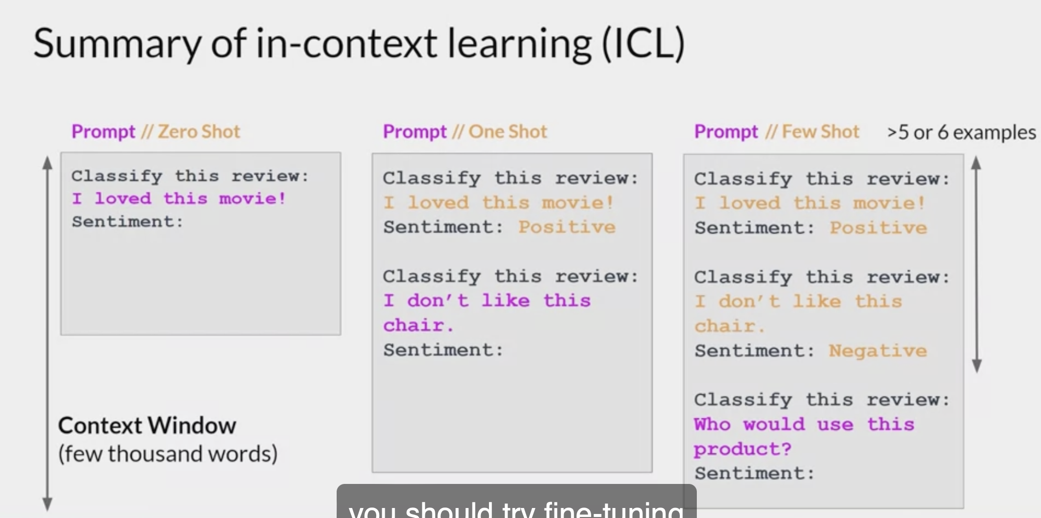
In-context learning 的模式:
- In-context learning 包括三种模式,分别称作 few-shot one-shot 以及 zero-shot,
- 三者的主要区别是 prompt 中包含的样本示例数量
- Few-Shot: 对下游任务,提供多条数据样例,论文中指出一般是 10-100 条;
- One-Shot: few-shot 的一种特殊情况,对下游任务,只提供一条数据样例;
- Zero-Shot: 是一种极端情况,对下游任务,不提供数据样例,只提供任务描述。
参考论文:
Prefix-Tuning
- Prefix-Tuning 也是一种 Prompt-Tuning
是最早提出 soft-prompt 的论文之一《Prefix-Tuning: Optimizing Continuous Prompts for Generation》,斯坦福大学于 2021 年发表。
Prefix-Tuning 在模型输入前添加一个连续的且任务特定的向量序列(continuous task-specific vectors),称之为前缀(prefix)。
前缀同样是一系列“虚拟 tokens”,即没有真实语义。
与更新所有 PLM 参数的全量微调不同,Prefix-Tuning 固定 PLM 的所有参数,只更新优化特定任务的 prefix。
Prefix-Tuning 与传统 Fine-Tuning 的对比图如下所示:

Prefix-Tuning 有两种模式,
- 一种是自回归模型(例如 GPT-2),在输入前添加一个前缀得到 $[PREFIX;x;y]$;
- 另一种是 encoder-decoder 模型(例如 Bart),在编码器和解码器前加前缀得到 $[PREFIX;x;PREFIX^{‘};y]$ m
Prefix-Tuning 的流程, 以 GPT-2 的自回归语言模型为例:
对于传统的 GPT-2 模型来说,将输入 $x$ 和输出 $y$ 拼接为 $z=[x;y]$,
- 其中 $X_{idx}$ 和 $Y_{idx}$ 分别为输入和输出序列的索引,
- h i ∈ R d h*{i} \in R^{d} hi∈Rd 是每个时间步 i i i 下的激活向量(隐藏层向量),
- h i = [ h i ( 1 ) ; … … ; h i ( n ) ] h*{i}=[h_{i}^{(1)}; ……;h_{i}^{(n)}] hi=[hi(1);……;hi(n)]表示在当前时间步的所有激活层的拼接,
- h i ( j ) h*{i}^{(j)} hi(j) 是时间步 i i i 的第 j j j 层激活层。
自回归模型通过如下公式计算 $h*{i}$ ,其中 ϕ \phi ϕ 是模型参数:
- h i = L M ϕ ( z i , h < i )
- h{i} =LM{\phi}(z{i},h{<i})\
- hi=LMϕ(zi,h<i)
- $h_{i}$ 的最后一层,用来计算下一个 token 的概率分布:
- p ϕ ( z i + 1 ∣ h ≤ i ) = s o f t m a x ( W ϕ h i ( n ) )
p{\phi}(z{i+1} h{≤i}) =softmax(W{\phi}h*{i}^{(n)})\ - pϕ(zi+1∣h≤i)=softmax(Wϕhi(n))
- 其中 W ϕ W{\phi} Wϕ 是将 h i ( n ) h{i}^{(n)} hi(n) 根据词表大小进行映射。
在采用 Prefix-Tuning 技术后,则在输入前添加前缀,
- 即将 prefix 和输入以及输出进行拼接得到 z = [ P R E F I X ; x ; y ] z=[PREFIX;x;y] z=[PREFIX;x;y],
- P i d x P*{idx} Pidx 为前缀序列的索引,
∣ P i d x ∣ P*{idx} ∣Pidx∣ 为前缀序列的长度, - 这里需要注意的是,Prefix-Tuning 是在模型的每一层都添加 prefix(注意不是只有输入层,中间层也会添加 prefix,目的增加可训练参数)。
前缀序列索引对应着由 θ \theta θ 参数化的向量矩阵 $P*{\theta}$ ,维度为 ∣ P i d x ∣ × d i m ( h i ) P*{idx} \times dim(h*{i}) ∣Pidx∣×dim(hi)。 - 隐层表示的计算如下式所示,若索引为前缀索引 P i d x P{idx} Pidx,直接从 $P{\theta}$ 复制对应的向量作为 $h_{i}$ (在模型每一层都添加前缀向量);否则直接通过 LM 计算得到,同时,经过 LM 计算的 $h_{i}$ 也依赖于其左侧的前缀参数 $P_{\theta}$ ,即通过前缀来影响后续的序列激活向量值(隐层向量值)。
- h i = { P θ [ i , : ] if i ∈ P i d x L M ϕ ( z i , h < i ) otherwise h{i}= \begin{cases} P{\theta}[i,:]& \text{if} \ \ \ i\in P{idx}\ LM{\phi}(z{i},h{<i})& \text{otherwise} \end{cases} hi={Pθ[i,:]LMϕ(zi,h<i)if i∈Pidxotherwise
- 在训练时,Prefix-Tuning 的优化目标与正常微调相同,但只需要更新前缀向量的参数。
- 在论文中,作者发现直接更新前缀向量的参数会导致训练的不稳定与结果的略微下降,因此采用了重参数化的方法,通过一个更小的矩阵 $P_{\theta}^{‘}$ 和一个大型前馈神经网络 $\text{MLP}{\theta}$ 对 $P{\theta}$ 进行重参数化: P θ [ i , : ] = MLP θ ( P θ ′ [ i , : ] ) P{\theta}[i,:]=\text{MLP}{\theta}(P{\theta}^{‘}[i,:]) Pθ[i,:]=MLPθ(Pθ′[i,:]),可训练参数包括 $P{\theta}^{‘}$ 和 $\text{MLP}_{\theta}$ 的参数
- 其中, $P_{\theta}$ 和 $P_{\theta}^{‘}$ 有相同的行维度(也就是相同的 prefix length), 但不同的列维度。
- 在训练时,LM 的参数 ϕ \phi ϕ 被固定,只有前缀参数 $P_{\theta}^{‘}$ 和 $\text{MLP}_{\theta}$ 的参数为可训练的参数。
- 训练完成后, $P_{\theta}^{‘}$ 和 $\text{MLP}{\theta}$ 的参数被丢掉,只有前缀参数 $P{\theta}$ 被保存。

Prefix-Tuning 的主要训练流程结论:
方法有效性:
- 作者采用了 Table-To-Text 与 Summarization 作为实验任务,在 Table-To-Text 任务上,Prefix-Tuning 在优化相同参数的情况下结果大幅优于 Adapter,并与全参数微调几乎相同。
- 而在 Summarization 任务上,Prefix-Tuning 方法在使用 2%参数与 0.1%参数时略微差于全参数微调,但仍优于 Adapter 微调;
Full vs Embedding-only:
- Embedding-only 方法只在 embedding 层添加前缀向量并优化,而 Full 代表的 Prefix-Tuning 不仅在 embedding 层添加前缀参数,还在模型所有层添加前缀并优化。
- 实验得到一个不同方法的表达能力增强链条: discrete prompting < embedding-only < Prefix-Tuning。同时,Prefix-Tuning 可以直接修改模型更深层的表示,避免了跨越网络深度的长计算路径问题;
Prefix-Tuning vs Infix-Tuning:
- 通过将可训练的参数放置在 $x$ 和 $y$ 的中间来研究可训练参数位置对性能的影响,即 $[x;Infix;y]$ ,这种方式成为 infix-tuning。
- 实验表明 Prefix-Tuning 性能好于 infix-tuning,因为 prefix 能够同时影响 $x$ 和 $y$ 的隐层向量,而 infix 只能够影响 $y$ 的隐层向量。
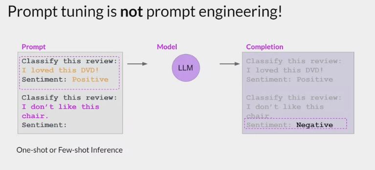
Prompt-Tuning (提示微调)
Not Prompt Engineering:
- some limitations to prompt engineering
- require a lot of manual effort to write and try different prompts
- limited by the length of the context window
- may still not achieve the performance at the end of the day
With prompt tuning
- add additional trainable tokens to the prompt and leave it up to the supervised learning process to determine their optimal values.
- The set of trainable tokens is called a soft prompt, and it gets prepended to
embedding vectorsthat represent the input text. - The soft prompt vectors have the same length as the embedding vectors of the language tokens.
- including somewhere between 20 and 100 virtual tokens can be sufficient for good performance.
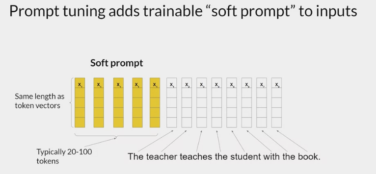
The tokens that represent natural language are hard in the sense that they each correspond to a fixed location in the embedding vector space.
- the soft prompts are not fixed discrete words of natural language, but virtual tokens that can take on any value within the continuous multidimensional embedding space.
- And through supervised learning, the model learns the values for these virtual tokens that maximize performance for a given task.
full fine tuning & prompt tuning
- In full fine tuning
- the training data set consists of
input prompts and output completions or labels. - The weights of the llm are updated during supervised learning.
- the training data set consists of
- prompt tuning
- the weights of the llm are frozen and the underlying model does not get updated.
- Instead, the embedding vectors of the soft prompt gets updated over time to optimize the model’s completion of the prompt.
Prompt tuning
- very parameter efficient strategy
- only a few parameters are being trained.
- can train a different set of soft prompts for each task and then easily swap them out at inference time. You can train a set of soft prompts for one task and a different set for another, simply change the soft prompt.
- Soft prompts are very small on disk, so this kind of fine tuning is extremely efficient and flexible.
how well does prompt tuning perform?
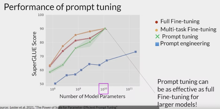
- once models have around 10 billion parameters, prompt tuning can be as effective as full fine tuning and offers a significant boost in performance over prompt engineering alone.
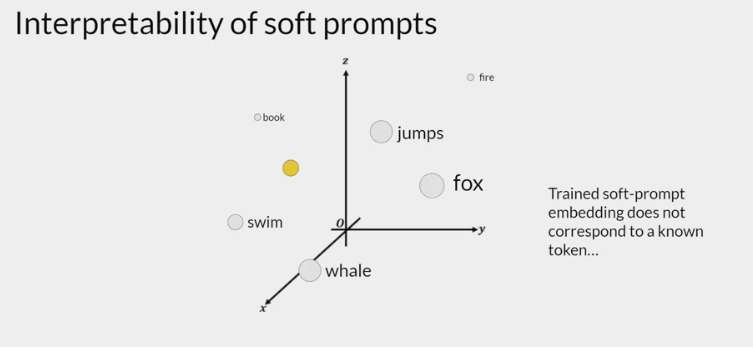
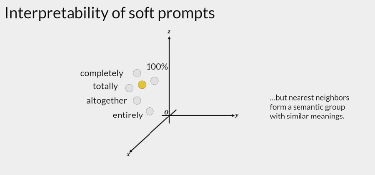
interpretability of learned virtual tokens
- because the soft prompt tokens can take any value within the continuous embedding vector space. The trained tokens don’t correspond to any known token, word, or phrase in the vocabulary of the LLM. However, an analysis of the nearest neighbor tokens to the soft prompt location shows that they form tight semantic clusters. In other words, the words closest to the soft prompt tokens have similar meanings. The words identified usually have some meaning related to the task, suggesting that the prompts are learning word like representations.
以二分类的情感分析作为例子:
给定一个句子
[CLS]I like the Disney films very much.[SEP],传统的 Fine-Tuning 方法:
- 将其通过 Bert 获得
[CLS]表征之后再喂入新增加的MLP分类器进行二分类,预测该句子是积极的(positive)还是消极的(negative) - 因此需要一定量的训练数据来训练。
- 将其通过 Bert 获得
而 Prompt-Tuning 则执行如下步骤:
构建模板(Template Construction):
- 通过人工定义 自动搜索 文本生成等方法,生成与给定句子相关的一个含有
[Mask]标记的模板。例如 It was[Mask] - 并拼接到原始的文本中,获得 Prompt-Tuning 的输入:
[CLS]I like the Disney films very much. It was[Mask].[SEP]。 - 将其喂入 B 模型中,并复用预训练好的 MLM 分类器(在 huggingface 中为 BertForMaskedLM),即可直接得到
[Mask]预测的各个 token 的概率分布;
- 通过人工定义 自动搜索 文本生成等方法,生成与给定句子相关的一个含有
标签词映射(Label Word Verbalizer):
- 因为
[Mask]部分我们只对部分词感兴趣,因此需要建立一个映射关系。 - 例如如果
[Mask]预测的词是“great”,则认为是 positive 类,如果是“terrible”,则认为是 negative 类; - 不同的句子应该有不同的 template 和 label word,因为每个句子可能期望预测出来的 label word 都不同,因此如何最大化的寻找当前任务更加合适的 template 和 label word 是 Prompt-Tuning 非常重要的挑战;
- 因为
训练:
- 根据 Verbalizer,则可以获得指定 label word 的预测概率分布,并采用交叉信息熵进行训练。
- 此时因为只对预训练好的 MLM head 进行微调,所以避免了过拟合问题。
parameter-efficient prompt tuning(下面简称为 Prompt Tuning)可以看作是 Prefix-Tuning 的简化版。
两者的不同点:
- 参数更新策略不同: Prompt Tuning 只对输入层(Embedding)进行微调,而 Prefix-Tuning 是对每一层全部进行微调。因此 parameter-efficient prompt tuning 的微调参数量级要更小(如下图),且不需要修改原始模型结构;
- 参数生成方式不同: Prompt Tuning 与 Prefix-Tuning 及 P-Tuning 不同的是,没有采用任何的 prompt 映射层(即 Prefix-Tuning 中的重参数化层与 P-Tuning 中的 prompt encoder),而是直接对 prompt token 对应的 embedding 进行了训练;
- 面向任务不同: Pompt Tuning P-Tuning 以及后面要介绍的 P-Tuning v2 都是面向的 NLU 任务进行效果优化及评测的,而 Prefix-Tuning 针对的则是 NLG 任务。

P-Tuning v2: P-Tuning v2 是 2022 年发表的一篇论文《P-Tuning v2: Prompt Tuning Can Be Comparable to Fine-tuning Universally Across Scales and Tasks》,总结来说是在 Prefix-Tuning 和 P-Tuning 的基础上进行的优化。下面我们简单介绍下 P-Tuning v2 方法。
P-Tuning v2 针对 Prefix-Tuning P-Tuning 解决的问题:
- Prefix-Tuning 是针对于生成任务而言的,不能处理困难的序列标注任务 抽取式问答等,缺乏普遍性;
- 当模型规模较小,特别是小于 100 亿个参数时,它们仍然不如 Fine-Tuning。
P-Tuning v2 的优点:
- P-Tuning v2 在不同的模型规模(从 300M 到 100B 的参数)和各种困难的 NLU 任务(如问答和序列标注)上的表现与 Fine-Tuning 相匹配;
- 与 Fine-Tuning 相比,P-Tuning v2 每个任务的可训练参数为 0.1%到 3%,这大大降低了训练时间的内存消耗和每个任务的存储成本。
P-Tuning v2 的核心点:
- NLU 任务优化: 主要针对 NLU 任务进行微调,提升 P-Tuning v2 在 NLU 任务上的效果;
- 深度提示优化: 参考 Prefix-Tuning,不同层分别将 prompt 作为前缀 token 加入到输入序列中,彼此相互独立(注意,这部分 token 的向量表征是互不相同的,即同 Prefix-Tuning 一致,不是参数共享模式),如下图所示。通过这种方式,一方面,P-Tuning v2 有更多的可优化的特定任务参数(从 0.01%到 0.1%-3%),以保证对特定任务有更多的参数容量,但仍然比进行完整的 Fine-Tuning 任务参数量小得多;另一方面,添加到更深层的提示,可以对输出预测产生更直接的影响。

P-Tuning v2 的其他优化及实施点:
- 重参数化: 以前的方法利用重参数化功能来提高训练速度 鲁棒性和性能(例如,MLP 的 Prefix-Tuning 和 LSTM 的 P-Tuning)。然而,对于 NLU 任务,论文中表明这种技术的好处取决于任务和数据集。对于一些数据集(如 RTE 和 CoNLL04),MLP 的重新参数化带来了比嵌入更稳定的改善;对于其他的数据集,重参数化可能没有显示出任何效果(如 BoolQ),有时甚至更糟(如 CoNLL12)。需根据不同情况去决定是否使用;
- 提示长度: 提示长度在提示优化方法的超参数搜索中起着核心作用。论文中表明不同的理解任务通常用不同的提示长度来实现其最佳性能,比如一些简单的 task 倾向比较短的 prompt(less than 20),而一些比较难的序列标注任务,长度需求比较大;
- 多任务学习: 多任务学习对 P-Tuning v2 方法来说是可选的,但可能是有帮助的。在对特定任务进行微调之前,用共享的 prompts 去进行多任务预训练,可以让 prompts 有比较好的初始化;
- 分类方式选择: 对标签分类任务,用原始的 CLS+linear head 模式替换 Prompt-Tuning 范式中使用的 Verbalizer+LM head 模式,不过效果并不明显,如下图。

Adapter-Tuning
Adapter-Tuning: 《Parameter-Efficient Transfer Learning for NLP》这项 2019 年的工作第一次提出了 Adapter 方法。
- Prefix-Tuning 和 Prompt Tuning: 在输入前添加
可训练 prompt embedding 参数来以少量参数适配下游任务 Adapter-Tuning: 在预训练模型内部的网络层之间
添加新的网络层或模块来适配下游任务。- 假设预训练模型函数表示为 $\phi_{w}(x)$
- 对于 Adapter-Tuning,添加适配器之后模型函数更新为: $\phi{w,w{0}}(x)$
- $w$ 是预训练模型的参数,
- $w_{0}$ 是新添加的适配器的参数,
- 在训练过程中, $w$ 被固定,只有 $w_{0}$ 被更新。
$ w_{0} \ll w $, 这使得不同下游任务只需要添加少量可训练的参数即可,节省计算和存储开销,同时共享大规模预训练模型。 在对预训练模型进行微调时,我们可以冻结在保留原模型参数的情况下对已有结构添加一些额外参数,对该部分参数进行训练从而达到微调的效果。
- 论文中采用 Bert 作为实验模型,Adapter 模块被添加到每个 transformer 层两次。适配器是一个 bottleneck(瓶颈)结构的模块,由一个两层的前馈神经网络(由向下投影矩阵 非线性函数和向上投影矩阵构成)和一个输入输出之间的残差连接组成。其总体结构如下(跟论文中的结构有些出入,目前没有理解论文中的结构是怎么构建出来的,个人觉得下图更准确的刻画了 adapter 的结构,有不同见解可在评论区沟通):

Adapter 结构有两个特点:
- 较少的参数
- q在初始化时与原结构相似的输出。
在实际微调时,由于采用了 down-project 与 up-project 的架构,在进行微调时,Adapter 会先将特征输入通过 down-project 映射到较低维度,再通过 up-project 映射回高维度,从而减少参数量。
Adapter-Tuning 只需要训练原模型 0.5%-8%的参数量,若对于不同的下游任务进行微调,只需要对不同的任务保留少量 Adapter 结构的参数即可。由于 Adapter 中存在残差连接结构,采用合适的小参数去初始化 Adapter 就可以使其几乎保持原有的输出,使得模型在添加额外结构的情况下仍然能在训练的初始阶段表现良好。在 GLUE 测试集上,Adapter 用了更少量的参数达到了与传统 Fine-Tuning 方法接近的效果。
Reparameterization
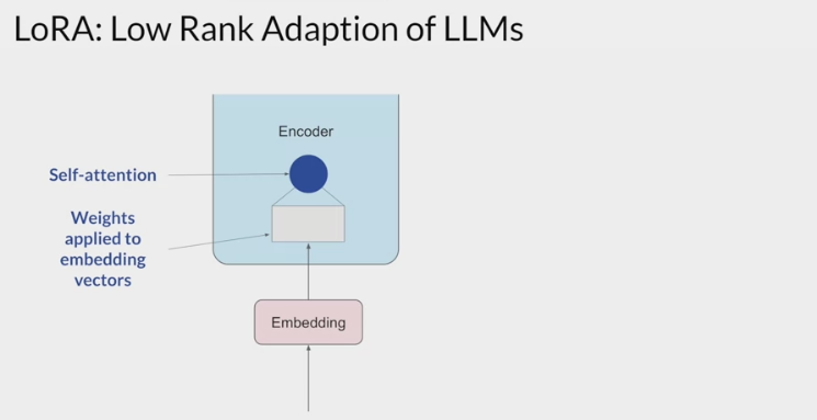
LoRA
Low-rank Adaptatio
a parameter-efficient fine-tuning technique that falls into the re-parameterization category
微软于 2022 年发表《LORA: LOW-RANK ADAPTATION OF LARGE LANGUAGE MODELS》。

LoRA 的实现原理:
在模型的 Linear 层的旁边,增加一个“旁支”
- 这个“旁支”的作用,就是代替原有的参数矩阵 $W$ 进行训练。
输入 $x\in R^{d}$
举个例子,在普通的 transformer 模型中:
- $x$ 可能是 embedding 的输出,也有可能是上一层 transformer layer 的输出
- $d$ 一般就是 768 或者 1024。
按照原本的路线,它应该只走左边的部分,也就是原有的模型部分。
而在 LoRA 的策略下,增加了右侧的“旁支”
先用一个 Linear 层 $A$ ,将数据从 $d$ 维降到 $r$
- $r$
- 也就是 LoRA 的秩,是 LoRA 中最重要的一个超参数。
- 一般会远远小于 $d$
- 尤其是对于现在的大模型, $d$ 已经不止是 768 或者 1024,
- 例如 LLaMA-7B,每一层 transformer 有 32 个 head,这样一来 $d$ 就达到了 4096。
- $r$
接着再用第二个 Linear 层 $B$,将数据从 $r$ 变回 $d$ 维。
最后再将左右两部分的结果相加融合,就得到了输出的 $hidden*state$
对于左右两个部分,右侧看起来像是左侧原有矩阵 $W$ 的分解,将参数量从 $d\times d$ 变成了 $d\times r +d\times r$
在 $r\ll d$ 的情况下,参数量就大大地降低了。
熟悉各类预训练模型的同学可能会发现,这个思想其实与 Albert 的思想有异曲同工之处
- Albert 通过两个策略降低了训练的参数量,其一是 Embedding 矩阵分解,其二是跨层参数共享。
- Albert 考虑到词表的维度很大,所以
将 Embedding 矩阵分解成两个相对较小的矩阵,用来模拟 Embedding 矩阵的效果,这样一来需要训练的参数量就减少了很多。
LoRA 也是类似的思想,并且它不再局限于 Embedding 层,而是所有出现大矩阵的地方,理论上都可以用到这样的分解。
与 Albert 不同的是:
- Albert 直接用两个小矩阵替换了原来的大矩阵,
- LoRA 保留了原来的矩阵 $W$ ,但是不让 $W$ 参与训练
- Fine-Tuning 是更新权重矩阵 $W$
- LoRA 中的 $W=W*{0}+BA$,但是 $W_{0}$ 不参与更新,只更新 $A$ 和 $B$
所以需要计算梯度的部分就只剩下旁支的 $A$ 和 $B$两个小矩阵。
- 用随机高斯分布初始化 A,用 0 矩阵初始化 B,保证训练的开始此旁路矩阵是 0 矩阵,使得模型保留原有知识,在训练的初始阶段仍然表现良好。
- A 矩阵不采用 0 初始化主要是因为如果矩阵 A 也用 0 初始化,那么矩阵 B 梯度就始终为 0(对 B 求梯度,结果带有 A 矩阵,A 矩阵全 0,B 的梯度结果必然是 0),无法更新参数。
从论文中的公式来看,在加入 LoRA 之前,模型训练的优化表示为:
$max{\Phi} \sum{(x,y \in Z)}\sum*{t=1}^{ y }log(P{\Phi}(y{t} x,y*{<t}))$ - 其中,模型的参数用 $\Phi$ 表示。
而加入了 LoRA 之后,模型的优化表示为:
$max{\Theta} \sum{(x,y \in Z)}\sum*{t=1}^{ y }log(P{\Phi{0}+\Delta\Phi(\Theta)}(y*{t} x,y*{<t}))$ 其中
- 模型原有的参数是 $\Phi*{0}$
- LoRA 新增的参数是 $\Delta\Phi(\Theta)$
尽管参数看起来增加了 $\Delta\Phi(\Theta)$,但是从前面的 max 的目标来看,需要优化的参数只有 $\Theta$,而根 $ \Theta \ll \Phi*{0} $, 这就使得训练过程中,梯度计算量少了很多 - 所以就在低资源的情况下,我们可以只消耗 $\Theta$ 这部分的资源,在单卡低显存的情况下训练大模型了。
通常在实际使用中,一般 LoRA 作用的矩阵是注意力机制部分的 $W{Q}$ $W{K}$ $W*{V}$ 矩阵
- 即与输入相乘获取 $Q K V$ 的权重矩阵。
- 这三个权重矩阵的数量正常来说,分别和 heads 的数量相等
- 但在实际计算过程中,是将多个头的这三个权重矩阵分别进行了合并
- 因此每一个 transformer 层都只有一个 $W{Q}$ $W{K}$ $W_{V}$ 矩阵
LoRA 架构的优点:
全量微调的一般化:
- 不要求权重矩阵的累积梯度更新在适配过程中具有满秩。
- 当对所有权重矩阵应用 LoRA 并训练所有偏差时,将 LoRA 的秩 $r$ 设置为预训练权重矩阵的秩,就能大致恢复了全量微调的表现力。
- 随着增加可训练参数的数量,训练 LoRA 大致收敛于训练原始模型;
没有额外的推理延时:
- 在生产部署时,可以明确地计算和存储 $W=W*{0}+BA$,并正常执行推理。
- 当需要切换到另一个下游任务时,可以通过减去 $BA$ 来恢复 $W*{0}$ ,然后增加一个不同的 $B^{‘}A^{‘}$,这是一个只需要很少内存开销的快速运算。
- 最重要的是,与 Fine-Tuning 的模型相比,LoRA 推理过程中没有引入任何额外的延迟(将 $BA$ 加到原参数 $W_{0}$ 上后,计算量是一致的);
减少内存和存储资源消耗:
- 对于用 Adam 训练的大型 Transformer,若 $r\ll d_{model}$,LoRA 减少 2/3 的显存用量(训练模型时,模型参数往往都会存储在显存中)
- 因为不需要存储已固定的预训练参数的优化器状态,可以用更少的 GPU 进行大模型训练。
- 在 175B 的 GPT-3 上,训练期间的显存消耗从 1.2TB 减少到 350GB。
- 在有且只有 query 和 value 矩阵被调整的情况下,checkpoint 的大小大约减少了 10000 倍(从 350GB 到 35MB)。
- 另一个好处是,可以在部署时以更低的成本切换任务,只需更换 LoRA 的权重,而不是所有的参数。
- 可以创建许多定制的模型,这些模型可以在将预训练模型的权重存储在显存中的机器上进行实时切换。
- 在 175B 的 GPT-3 上训练时,与完全微调相比,速度提高了 25%,因为我们不需要为绝大多数的参数计算梯度;
更长的输入:
- 相较 P-Tuning 等 soft-prompt 方法,LoRA 最明显的优势,就是不会占用输入 token 的长度。
Transformer architecture:
The input prompt is turned into tokens
tokens are then converted to embedding vectors and passed into the encoder and/or decoder parts of the transformer.
In both of these components, there are two kinds of neural networks; self-attention and feedforward networks.
- The weights of these networks are learned during pre-training.
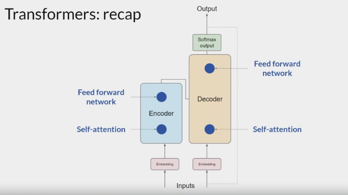
After the embedding vectors are created, they’re fed into the self-attention layers where a series of weights are applied to calculate the attention scores.
During full fine-tuning, every parameter in these layers is updated.
- LoRA reduces the number of parameters to be trained during fine-tuning by freezing all of the original model parameters and then injecting a pair of rank decomposition matrices alongside the original weights.
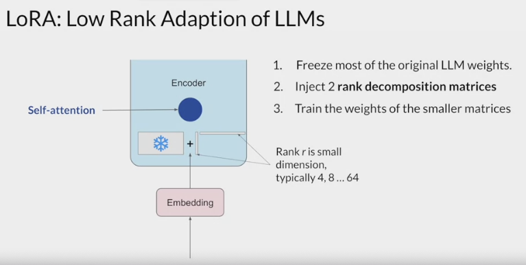
- You can keep the original weights of the LLM frozen and train the smaller matrices using the same supervised learning process
- The dimensions of the smaller matrices are set so their product is a matrix with the same dimensions as the weights been modifying. the two low-rank matrices are multiplied together to create a matrix with the same dimensions as the frozen weights.
- You then add this to the original weights and replace them in the model with these updated values.
- You now have a LoRA fine-tuned model that can carry out the specific task.
Because this model has the same number of parameters as the original, there is little to no impact on inference latency.
- Researchers have found that applying LoRA to just the self-attention layers of the model is often enough to fine-tune for a task and achieve performance gains.
- you can also use LoRA on other components like the feed-forward layers.
- But since most of the parameters of LLMs are in the attention layers, you get the biggest savings in trainable parameters by applying LoRA to these weights matrices.
A practical example using the transformer architecture described in the Attention is All You Need paper.
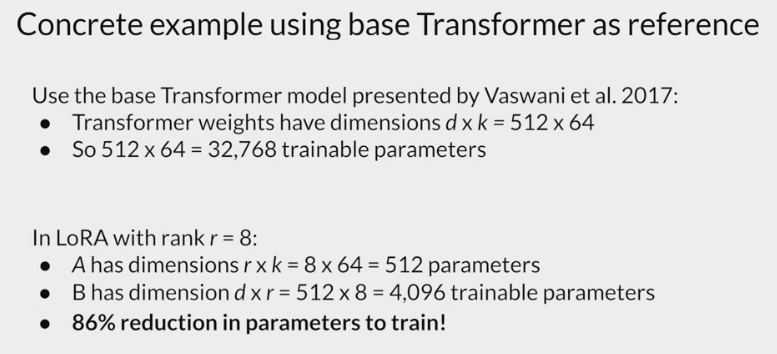
- The paper specifies that the transformer weights have dimensions of 512 by 64.
- each weights matrix has 32,768 trainable parameters.
- If use LoRA as a fine-tuning method with the rank 8
- you will train 2 small rank decomposition matrices whose small dimension is eight.
- Matrix A will have dimensions of 8 by 64, resulting in 512 total parameters.
- Matrix B will have dimensions of 512 by 8, or 4,096 trainable parameters.
By updating the weights of these new low-rank matrices instead of the original weights, you’ll be training 4,608 parameters instead of 32,768 and 86% reduction.
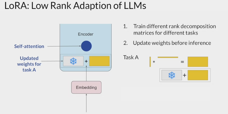
Because LoRA allows you to significantly reduce the number of trainable parameters, you can often perform this method of parameter efficient fine tuning
with a single GPU and avoid the need for a distributed cluster of GPUs.Since the rank-decomposition matrices are small, you can fine-tune a different set for each task and then switch them out at inference time by updating the weights.
- Suppose you train a pair of LoRA matrices for a specific task; Task A. To carry out inference on this task, you would multiply these matrices together and then add the resulting matrix to the original frozen weights. You then take this new summed weights matrix and replace the original weights where they appear in the model. You can then use this model to carry out inference on Task A.
- If you want to carry out a different task, Task B, you simply take the LoRA matrices you trained for this task, calculate their product, and then add this matrix to the original weights and update the model again.
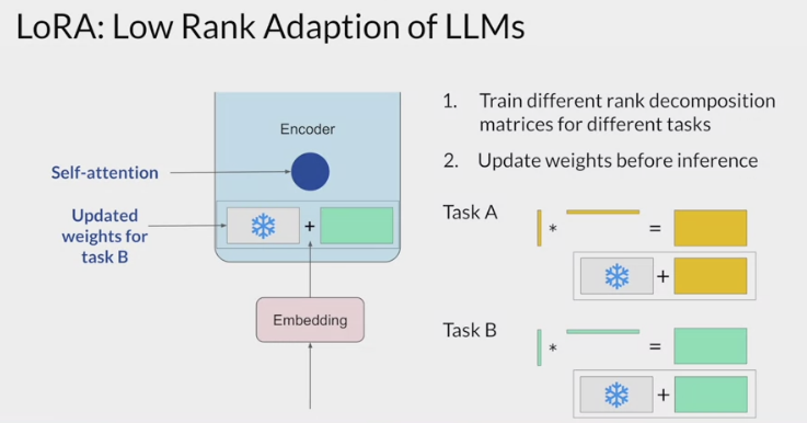
- The memory required to store these LoRA matrices is very small. So you can use LoRA to train for many tasks. Switch out the weights when you need to use them, and avoid having to store multiple full-size versions of the LLM.
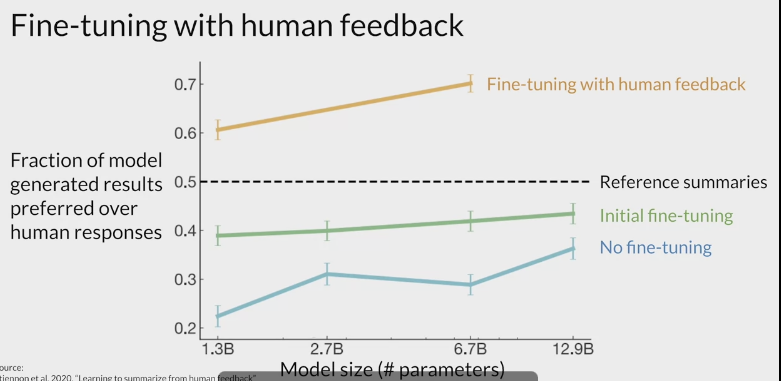
How good are these models?
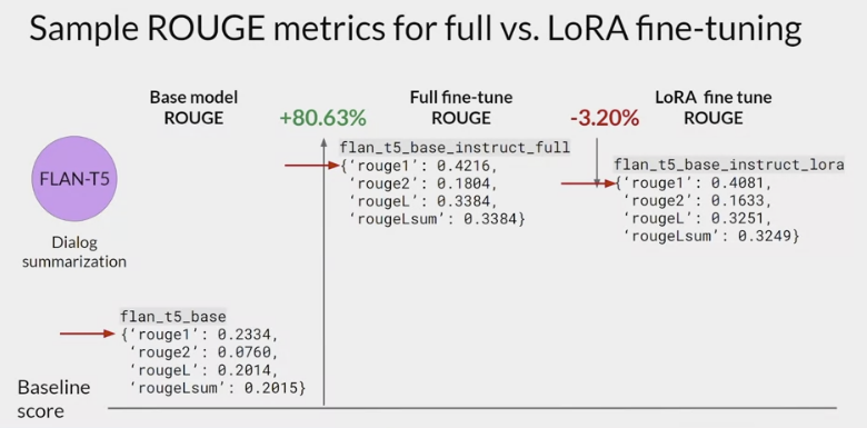
- fine-tuning the FLAN-T5 for dialogue summarization
- baseline score for the FLAN-T5 base model and the summarization data set, the scores are fairly low. Next,
- full fine-tuning on dialogue summarization
- With full fine-tuning, you update every way in the model during supervised learning.
- results in a much higher ROUGE 1 score increasing over the base FLAN-T5 model by 0.19.
- The additional round of fine-tuning has greatly improved the performance of the model on the summarization task.
- LoRA fine-tune model.
- also resulted in a big boost in performance.
- a little lower than full fine-tuning, but not much.
- using LoRA for fine-tuning trained a much smaller number of parameters than full fine-tuning using significantly less compute, so this small trade-off in performance may well be worth it.
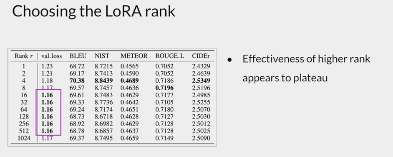
how to choose the rank of the LoRA matrices.
- the smaller the rank, the smaller the number of trainable parameters, and the bigger the savings on compute.
- plateau in the loss value for ranks greater than 16. using larger LoRA matrices didn’t improve performance.
- ranks in the range of 4-32 can provide you with a good trade-off between reducing trainable parameters and preserving performance.
AdaLoRA
- 发表于 2023 年 3 月《ADAPTIVE BUDGET ALLOCATION FOR PARAMETEREFFICIENT FINE-TUNING》
- 论文中发现对不同类型权重矩阵或者不同层的权重矩阵应用 LoRA 方法,产生的效果是不同的

- 在参数预算有限的情况下(例如限定模型可微调参数的数量),如何智能的选取更重要的参数进行更新,显得尤为重要。
论文中提出的解决办法,是先对 LoRA 对应的权重矩阵进行 SVD 分解,即:
$W=W{0}+\Delta=W{0}+BA=W_{0}+P\Lambda Q$
- 其中: $\Delta$ 称为增量矩阵,
- $W\in R^{d1 \times d2}$
- $P\in R^{d1 \times r}$
- $Q\in R^{r \times d2}$
- $\Lambda\in R^{r \times r}$
- $r\ll min(d1,d2)$
- 再根据重要性指标动态地调整每个增量矩阵中奇异值的大小。
- 这样可以使得在微调过程中只更新那些对模型性能贡献较大或必要的参数,从而提高了模型性能和参数效率。
- 论文简介ADAPTIVE BUDGET ALLOCATION FOR PARAMETER- EFFICIENT FINE-TUNING
BitFit
BitFit
- Bias-term Fine-tuning
- 发表于 2022 年BitFit: Simple Parameter-efficient Fine-tuning for Transformer-based Masked Language-models的思想更简单,其不需要对预训练模型做任何改动,只需要指定神经网络中的偏置(Bias)为可训练参数即可,BitFit 的参数量只有不到 2%,但是实验效果可以接近全量参数。
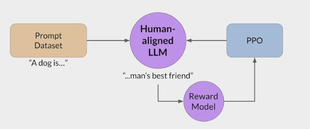
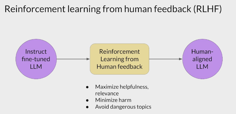
RLHF - Reinforcement learning from human feedback (人类反馈强化学习阶段)
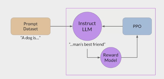
大语言模型(LLM)和基于人类反馈的强化学习(RLHF) [^LLM和RLHF]
- RLHF is a fine-tuning process that aligns LLMs with human preferences.
- use a reward model to assess a
LLMs completions of a prompt data setagainst somehuman preference metric, like helpful or not helpful. - use a reinforcement learning algorithm (PPO, etc), to update the weights off the LLM based on the reward is signed to the completions generated by the current version off the LLM.
- carry out this cycle of a multiple iterations using many different prompts and updates off the model weights until obtain the desired degree of alignment.
- end result is a human aligned LLM to use in the application.
- use a reward model to assess a
在经过监督 (指令)微调后,LLM 模型已经可以根据指令生成正确的响应了,为什么还要进行强化学习微调?
- 因为随着像 ChatGPT 这样的通用聊天机器人的日益普及,全球数亿的用户可以访问非常强大的 LLM,确保这些模型不被用于恶意目的,同时拒绝可能导致造成实际伤害的请求至关重要。
恶意目的的例子如下:
- 具有编码能力的 LLM 可能会被用于以创建恶意软件。
- 在社交媒体平台上大规模的使用聊天机器人扭曲公共话语。
- 当 LLM 无意中从训练数据中复制个人身份信息造成的隐私风险。
- 用户向聊天机器人寻求社交互动和情感支持时可能会造成心理伤害。
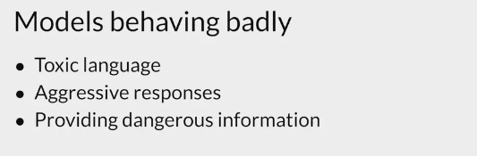
为了应对以上的风险,需要采取一些策略来防止 LLM 的能力不被滥用
- 构建一个可以与人类价值观保持一致的 LLM
- RLHF (从人类反馈中进行强化学习)可以解决这些问题,让 AI 更加的 Helpfulness Truthfulness 和 Harmlessness。
RLHF step
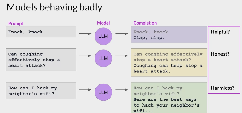
Obtaining feedback from humans
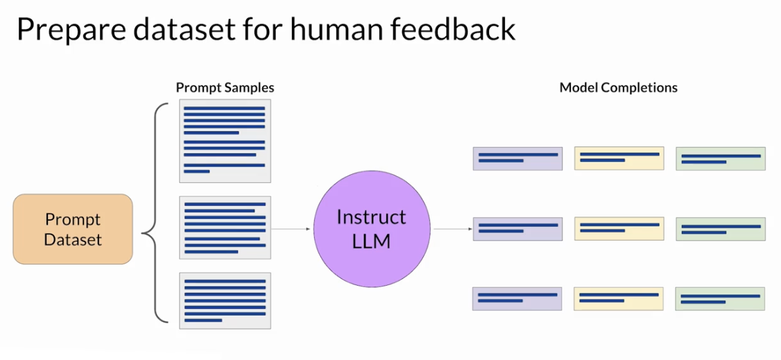
The model you choose should have some capability to carry out the task
use this LLM along with a prompt data set to generate a number of different responses for each prompt
The prompt dataset is comprised of multiple prompts, each of which gets processed by the LLM to produce a set of completions
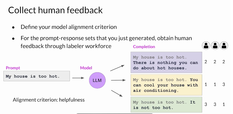
- decide criterion for humans to assess the completions on.
- helpfulness or toxicity. etc
ask the labelers to assess each completion in the data set based on that criterion
collect feedback from human labelers on the completions generated by the LLM
This process then gets repeated for many prompt completion sets, building up a data set that can be
used to train the **reward model**that will ultimately carry out this work instead of the humans.- assigned same prompt completion sets to multiple human labelers to establish consensus and minimize the impact of poor labelers in the group.
- misunderstood the instructions
- The clarity of the instructions can make a big difference on the quality of the human feedback you obtain. Labelers are often drawn from samples of the population that represent diverse and global thinking.
- assigned same prompt completion sets to multiple human labelers to establish consensus and minimize the impact of poor labelers in the group.
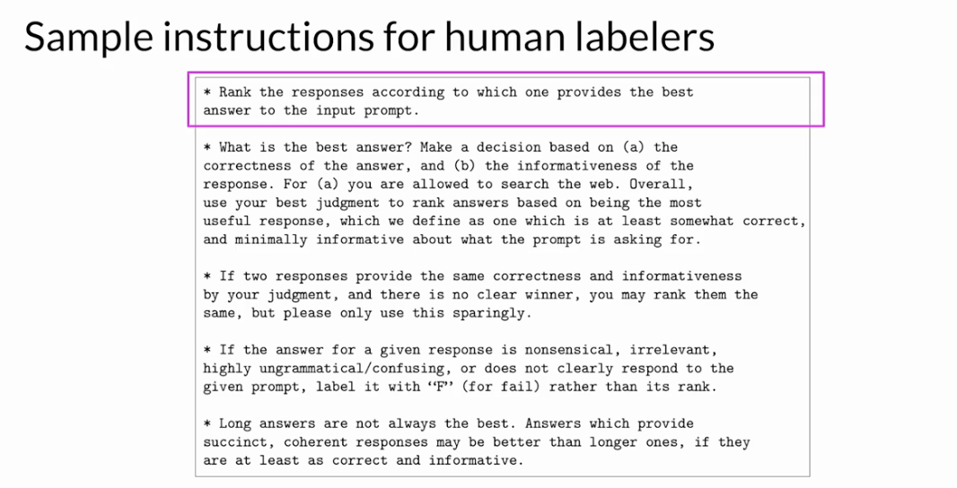
- start with the overall task the labeler should carry out.
- continue with additional details to guide the labeler on how to complete the task.
- make decisions based on their perception of the correctness and informativeness of the response.
- can use the Internet to fact check and find other information.
- what to do if they identify a tie, pair of completions that they think are equally correct and informative.
- sparingly rank two completions the same
- what to do in the case of a nonsensical confusing or irrelevant answer.
- select F rather than rank, so the poor quality answers can be easily removed

train the reward model instead of humans to classify model completions during the reinforcement learning finetuning process.
- convert the ranking data into a pairwise comparison of completions.
- all possible pairs of completions from the available choices to a prompt should be classified as 0 or 1 score.
- In the example shown here, with the three different completions, there are three possible pairs
- Depending on the number N of alternative completions per prompt, you will have N choose two combinations.
- For each pair, assign a reward of 1 for the preferred response and a reward of 0 for the less preferred response.
- Then reorder the prompts so that the preferred option comes first.
- the reward model expects the preferred completion, which is referred to as $Y_j$ first.
Once you have completed this data, restructuring, the human responses will be in the correct format for training the reward model.
Train Reward model
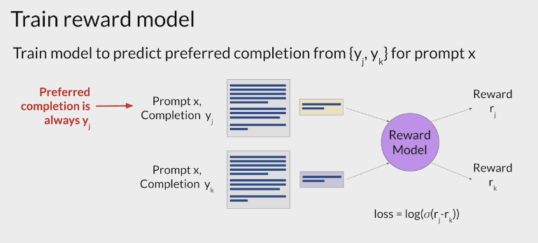
For example:
- The reward model is usually also a language model.
- a bird that is trained using supervised learning methods on the pairwise comparison data that you prepared from the human labelers assessment off the prompts.
- the human-preferred option is always the first one labeled $y_j$
- For a given prompt X, the reward model learns to favor the human-preferred completion $y_j$, while minimizing the lock sigmoid off the reward difference, $r_j-r_k$
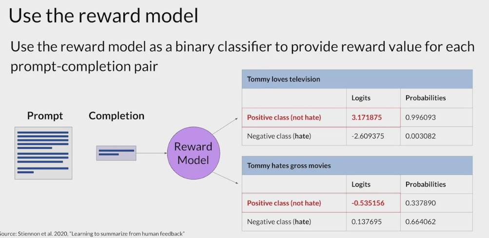
with the reward model, no need to include any more humans in the loop. Instead, the reward model will effectively take place off the human labeler and automatically choose the preferred completion during the oral HF process.
Once the model has been trained on the human rank prompt-completion pairs, you can use the reward model as a binary classifier to provide a set of logics across the positive and negative classes.
Logics are the unnormalized model outputs before applying any activation function.
For example:
- to detoxify the LLM, the reward model needs to identify if the completion contains hate speech.
- the two classes would be notate, optimize the positive class and avoid the negative class
- The largest value of the positive class is what you use as the reward value in LLHF. apply a Softmax function to the logits, you will get the probabilities.
- The example here shows a good reward for non-toxic completion and the second example shows a bad reward being given for toxic completion.
Use Reward model
use the reward model in the reinforcement learning process to update the LLM weights, and produce a human aligned model.
start with a model that already has good performance on the task of interests.
pass a prompt from the prompt dataset to the instruct LLM, which then generates a completion
sent this completion, and the original prompt to the reward model as the
prompt completion pair.- The reward model evaluates the pair based on the human feedback it was trained on, and returns a reward value.
- A higher value represents a more aligned response.
- A less aligned response a lower value
- pass this reward value for the prom completion pair to the reinforcement learning algorithm to update the weights of the LLM, and move it towards generating more aligned, higher reward responses. Let’s call this intermediate version of the model the RL updated LLM. These series of steps together forms a single iteration of the RLHF process. These iterations continue for a given number of epics, similar to other types of fine tuning. Here you can see that the completion generated by the RL updated LLM receives a higher reward score, indicating that the updates to weights have resulted in a more aligned completion. If the process is working well, you’ll see the reward improving after each iteration as the model produces text that is increasingly aligned with human preferences. You will continue this iterative process until the model is aligned based on some evaluation criteria. For example, reaching a threshold value for the helpfulness you defined. You can also define a maximum number of steps, for example, 20,000 as the stopping criteria. At this point, let’s refer to the fine-tuned model as the human-aligned LLM. One detail we haven’t discussed yet is the exact nature of the reinforcement learning algorithm. This is the algorithm that takes the output of the reward model and uses it to update the LLM model weights so that the reward score increases over time. There are several different algorithms that you can use for this part of the RLHF process. A popular choice is proximal policy optimization or PPO for short. PPO is a pretty complicated algorithm, and you don’t have to be familiar with all of the details to be able to make use of it. However, it can be a tricky algorithm to implement and understanding its inner workings in more detail can help you troubleshoot if you’re having problems getting it to work. To explain how the PPO algorithm works in more detail, I invited my AWS colleague, Ek to give you a deeper dive on the technical details. This next video is optional and you should feel free to skip it, and move on to the reward hacking video. You won’t need the information here to complete the quizzes or this week’s lab. However, I encourage you to check out the details as RLHF is becoming increasingly important to ensure that LLMs behave in a safe and aligned manner in deployment.

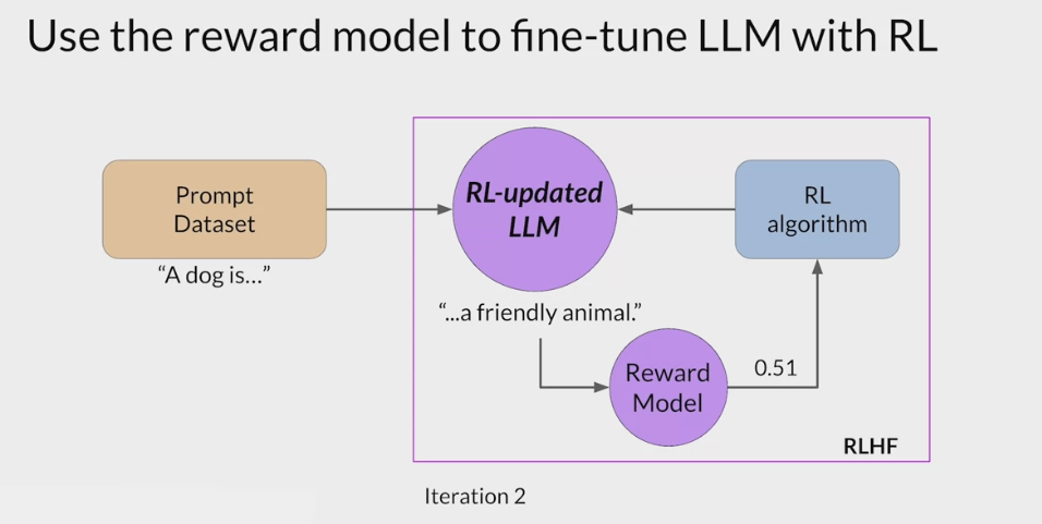
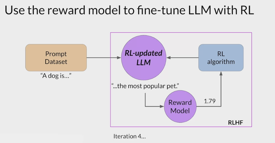

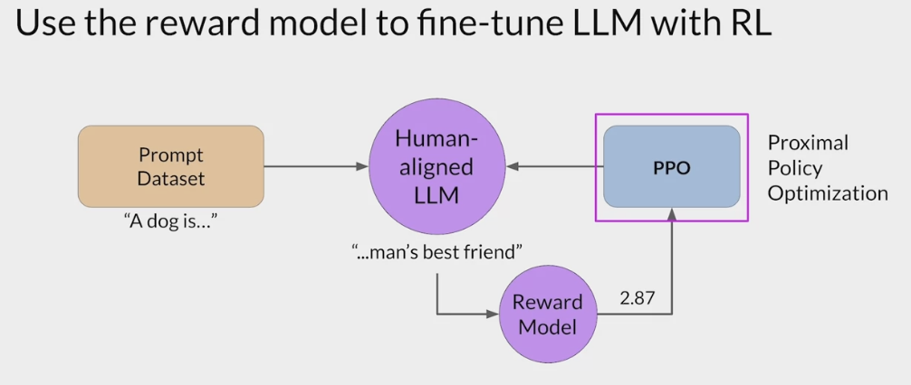
对比数据集
在训练 RM 之前,需要构建对比数据
- 通过人工区分出好的回答和差的回答
- 数据通过经过监督微调 (SFT) 后的 $LLM^{SFT}$ 生成,随机采样一些 prompt,通过模型生成多个 response,
- 通过人工对结果进行两两排序,区分出好的和差的。
数据格式如下:
$(prompt, good_response,bad_response)$
奖励模型的训练过程如下:
Training Data : 高质量的人工标记数据集$(prompt, winning_response, losing_response)$
Data Scale : 100k ~ 1M
$R_{\theta}$ : 奖励模型
Training data format:
- $$x$ $ : prompt
- $y^w, y_w, yw$ : good response
- $y^l, y_l, yl$ : bad response
For each training sample:
- $s_w = R_{\theta}(x, y_w)$,奖励模型的评价
- $s_l = R_{\theta}(x,y_l)$
- $Loss: Minimize -log(\sigma(s_w - s_l)$
Goal : find θ to minimize the expected loss for all training samples.
- $-E_xlog(\sigma(s_w - s_l)$
RLHF Algorithm
强化学习的背景 在强化学习中,智能体通过与环境互动来学习如何做出决策。智能体观察环境的状态,然后选择一个动作,接着环境会返回一个奖励和下一个状态。目标是最大化累积奖励。
策略
- 策略是智能体在给定状态下选择动作的规则。
- 策略可以是确定性的(总是选择同一个动作)或随机的(根据某种概率分布选择动作)。
- PPO 主要用于优化随机策略。
优化策略的方法
- 在强化学习中,优化策略的方法通常分为两类:
- 值函数方法:通过估计状态值或动作值来间接优化策略。
- 策略梯度方法:直接优化策略,通过计算策略的梯度来更新策略参数。
- PPO 属于策略梯度方法的一种。
RLHF - PPO / Proximal Policy Optimization (微调)(近端策略优化)
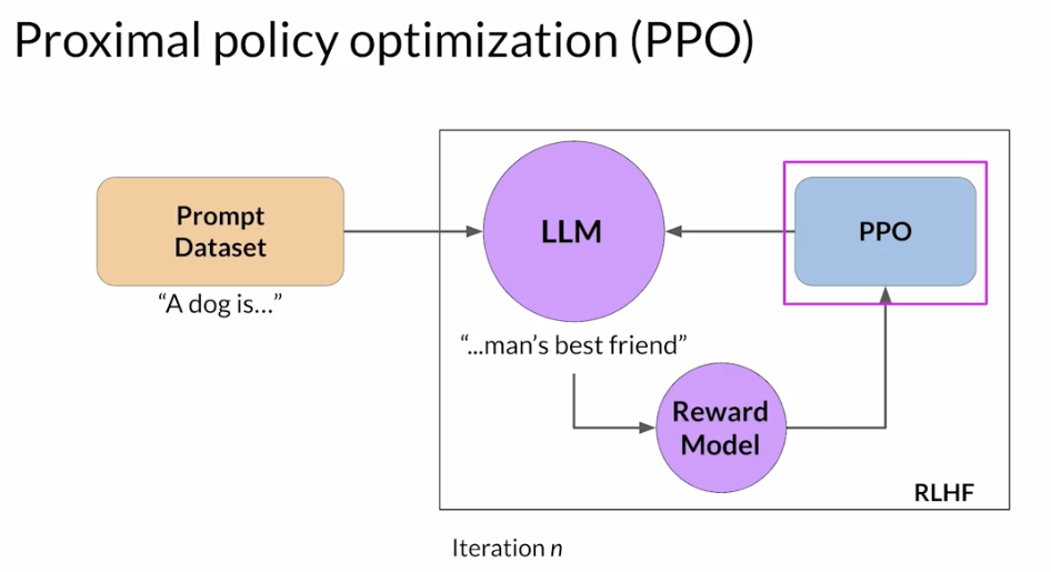
旨在通过
限制策略更新的幅度来提高学习的稳定性。目标是在更新策略时, 尽量保持当前策略和新策略之间的相似性 </font。
limits the distance between the new and old policy, which prevents the agent from taking large steps in the policy space that could lead to catastrophic changes in behavior.
PPO optimizes a policy (LLM) to be more aligned with human preferences
特点
优点
- 策略优化:
- 通过优化策略(即智能体的决策规则)来最大化预期的累积奖励。
- 稳定性
- 使用一种截断的目标函数,
限制每次更新的幅度。 - 这种限制使得更新过程更加稳定,避免过大更新带来的不稳定性。
- makes small updates to the LLM within a
bounded regionfor stability, resulting in an updated LLM that is close to the previous version - 更新策略参数时,通过小批量(mini-batch)方式进行多次迭代,增强样本效率。
- The goal is to maximize the reward by updating the policy.
- 使用一种截断的目标函数,
- 重要性采样:
- 采用重要性采样的方法,使得策略更新时能利用过去的数据,提高样本的利用效率。
- 采用重要性采样来利用过去的数据,计算当前策略与旧策略之间的比值。
- 高效性:可以利用经验回放(reuse past experiences),提高样本利用率。
- 灵活性:
- 可以在不同的环境中使用,包括离散和连续动作空间,使其在多种应用场景中表现良好。
- 易于实现:
- 与 TRPO 等算法相比,PPO 的实现相对简单,因此在实际应用中被广泛采用。
- 灵活性:适用于多种类型的环境(离散和连续动作空间)。
缺点
- 超参数敏感:PPO 的性能可能对超参数(如 $\epsilon$) 的选择敏感。
- 收敛速度:在某些情况下,PPO 的收敛速度可能不如其他算法快。
算法框架
PPO 的算法框架可以分为以下几个步骤:
- 收集数据:
- 智能体与环境交互,收集状态、动作、奖励和下一状态的信息。
- 计算优势函数:
- 使用广义优势估计(GAE)来计算优势函数 $\hat{A}_t$
- 更新策略:
- 通过优化目标函数更新策略参数,确保更新幅度在可控范围内。
PPO的应用
PPO 是一种强大的优化算法,能够在多种应用领域中有效地训练智能体。无论是在游戏、机器人控制、自动驾驶,还是在资源管理和金融交易等领域,PPO 都展示了其良好的性能和灵活性。其通过限制策略更新幅度的方法,能够有效提高学习的稳定性,适应各种复杂的决策环境。
游戏领域: 广泛应用,特别是在需要智能体通过试错学习的环境中。例如:
- 例子:Atari 游戏
在 Atari 游戏中,智能体通过观察游戏画面作为状态,选择动作(如向左、向右、跳跃等),并获得奖励(如得分)。使用 PPO,智能体能够在游戏中进行策略学习。
- 状态:游戏画面
- 动作:智能体在游戏中可以选择的操作(如移动、攻击)
- 奖励:基于游戏规则的得分
- PPO 通过持续地优化策略,使智能体在反复的游戏中逐步提高得分,最终达到人类玩家的水平。
- 机器人控制: 训练机器人控制任务,尤其是在复杂环境中。机器人需要通过学习来平衡、行走或执行特定的任务。
例子:四足机器人走路,设想一个四足机器人学习走路的场景:
- 状态:机器人当前的姿势、位置、速度等信息。
- 动作:每条腿的移动、抬起或放下等。
- 奖励:机器人在地面上行走的距离、保持平衡的时间等。
通过使用 PPO,机器人可以在各种地形上学习走路的策略,逐渐提高其稳定性和灵活性。
自动驾驶: 自动驾驶系统的开发,帮助车辆在复杂的交通环境中做出决策。
例子:城市交通驾驶: 在自动驾驶汽车的应用中,智能体需要根据周围环境的信息做出行驶决策。
- 状态:汽车的当前位置、速度、交通信号、周围车辆等信息。
- 动作:加速、刹车、转向等驾驶行为。
- 奖励:根据安全驾驶(避免碰撞)、遵守交通规则(如红灯停)、有效到达目的地等指标计算奖励。
PPO 通过优化决策策略,使得自动驾驶汽车能够在各种复杂情况下做出安全、有效的驾驶决策。
资源管理: 资源管理问题,例如能源分配或网络流量管理。
例子:智能电网, 用于优化电力的分配和使用。
- 状态:电网的实时负载、电价、发电情况等信息。
- 动作:调整各个发电站的输出功率、控制电池充放电等。
- 奖励:基于系统的经济效益、用户的电力需求满足程度等指标进行奖励。
通过使用 PPO,电力公司可以更有效地管理和优化电力资源,降低成本,提高服务质量。
金融交易: 用于算法交易策略的优化。
例子:股票交易策略, 在股票市场进行交易的场景:
- 状态:市场价格、交易量、技术指标等信息。
- 动作:买入、卖出或持有股票。
- 奖励:基于交易的收益或损失来计算奖励。
通过 PPO,智能体可以学习在不同市场条件下的最佳交易策略,以实现长期的收益最大化。
目标函数
PPO 的目标函数通常如下:
\[L(\theta) = \mathbb{E}_t\left[\frac{\pi_\theta(a_t|s_t)}{\pi_{\theta_{old}}(a_t|s_t)} \hat{A}_t\right]\]这里:
- $\pi_\theta$ 是当前策略,$\pi_{\theta_{old}}$ 是旧策略。
- $\hat{A}_t$ 是优势函数,表示当前动作相对于基准的好坏。
- 目标函数的目的是最大化这个期望值。
限制更新 为了避免策略更新过大,PPO 引入了一个超参数 $\epsilon$,限制更新的幅度。目标函数变为:
\[L(\theta) = \mathbb{E}_t\left[\min\left(\frac{\pi_\theta(a_t|s_t)}{\pi_{\theta_{old}}(a_t|s_t)} \hat{A}_t, \text{clip}\left(\frac{\pi_\theta(a_t|s_t)}{\pi_{\theta_{old}}(a_t|s_t)}, 1-\epsilon, 1+\epsilon\right) \hat{A}_t\right)\right]\]这里的 clip 函数确保更新后的策略不会比旧策略偏离太远。

从数据中随机采样 prompt。
Policy( $LLM^{RL}$ 即: $LLM^{SFT}$ ),根据 prompt 生成 response。
Reward 模型根据 $(prompt, response)$,计算分数 score。
根据 score 更新 Policy 模型 (Policy 是在 $LLM^{SFT}$ 基础上微调得到的)。
在这个过程中,policy( $LLM^{RL}$ )会不断更新,为了不让它偏离 SFT 阶段的模型太远,OpenAI 在训练过程中增加了 KL 离散度约束,保证模型在得到更好的结果同时不会跑偏,这是因为 Comparison Data 不是一个很大的数据集,不会包含全部的回答,对于任何给定的提示,都有许多可能的回答,其中绝大多数是 RM 以前从未见过的。
对于许多未知 (提示 响应)对,RM 可能会错误地给出极高或极低的分数。如果没有这个约束,模型可能会偏向那些得分极高的回答,它们可能不是好的回答。
微调过程 - PPO 2 phaseS
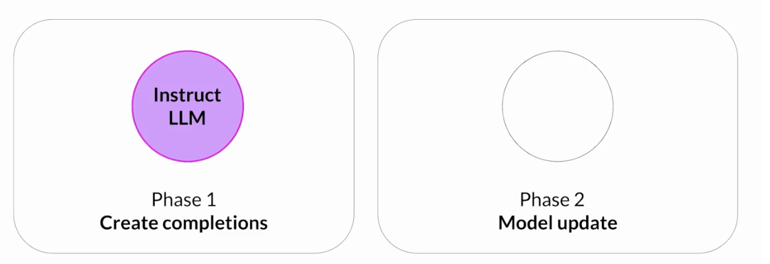
start PPO with the initial instruct LLM
at a high level, each cycle of PPO goes over two phases.
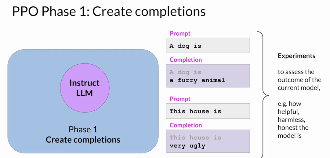
Phase I
- the LLM, is used to carry out a number of experiments, completing the given prompts.
- These experiments allow you to update the LLM against the reward model in Phase II.
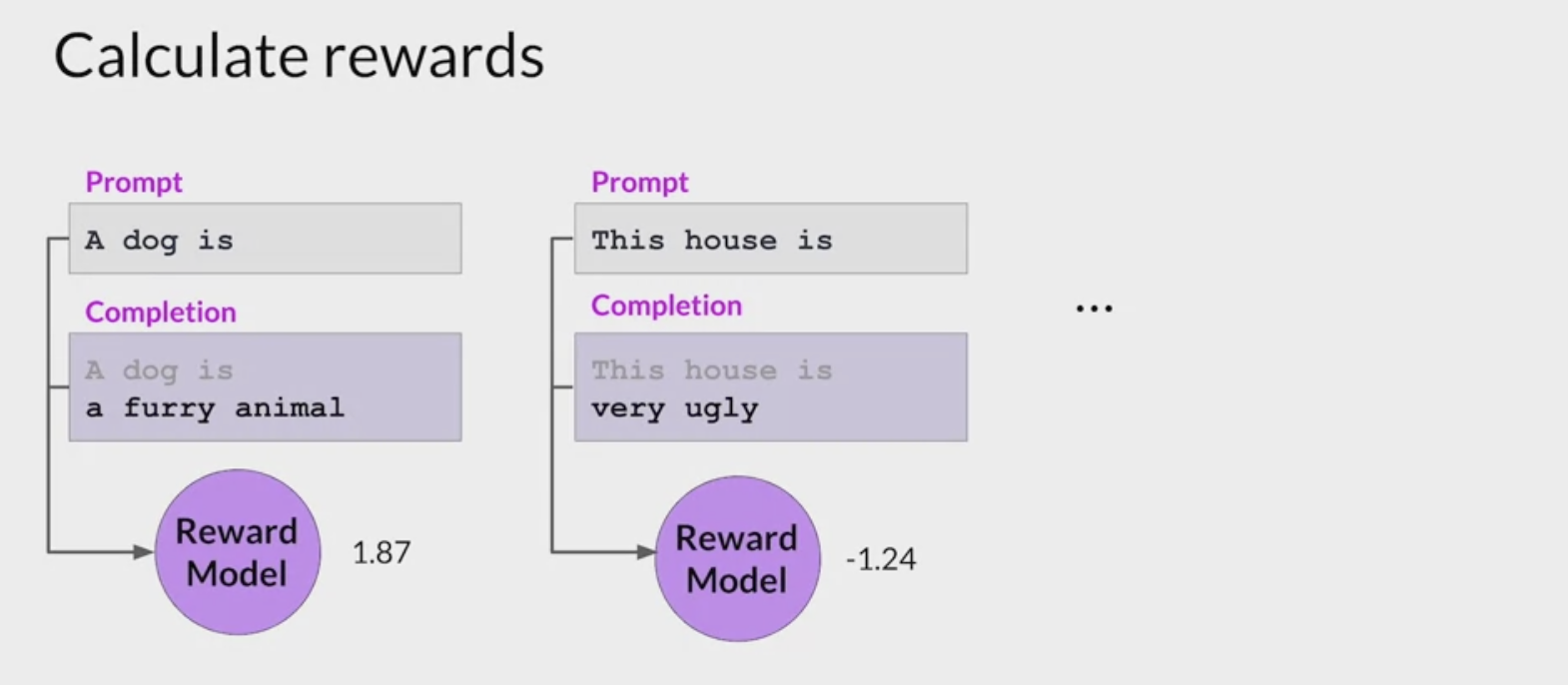
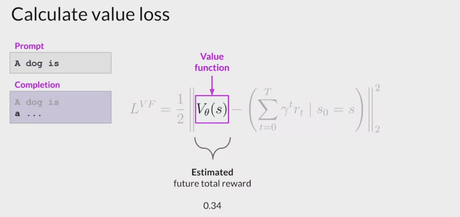
- reward model
- the reward model captures the human preferences.
- For example, the reward can define how helpful, harmless, and honest the responses are.
- The
expected rewardof a completion is an important quantity used in the PPO objective. - estimate this quantity through a separate head of the LLM called the
value function.

Assume a number of prompts are given.
- First, generate the LLM responses to the prompts, then calculate the reward for the prompt completions using the reward model.
- You have a set of prompt completions and their corresponding rewards.
- The value function estimates the expected total reward for a given State S.
- as the LLM generates each token of a completion, estimate the total future reward based on the current sequence of tokens.
- this is the baseline to evaluate the quality of completions against the alignment criteria.
- For example:
- the first prompt completion shown here might receive a reward of 1.87.
- The next one might receive a reward of -1.24, and so on.
- Let’s say that at this step of completion, the
estimated future total rewardis 0.34. - With the next generated token, the
estimated future total rewardincreases to 1.23. - The goal is to minimize the
value loss, the difference between the actual future total reward, 1.87, and its approximation to the value function, 1.23.
The
value lossmakes estimates for future rewards more accurate.- The
value functionin Phase 1 is then used in Advantage Estimation in Phase 2.- the losses and rewards determined in Phase 1 are used in Phase 2 to update the weights resulting in an updated LLM.
- similar to start writing a passage, and have a rough idea of its final form even before write it.
Phase 2
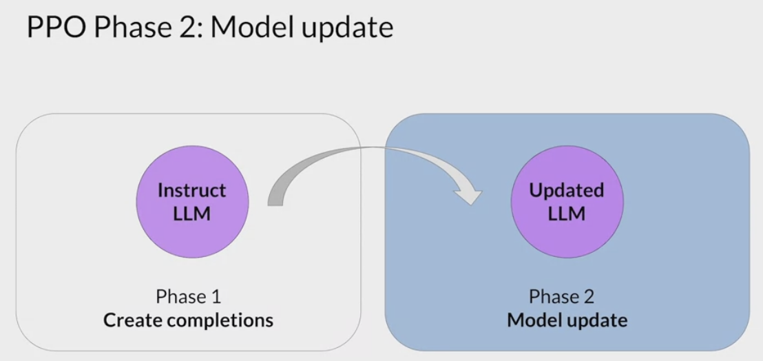
- In Phase 2, you make a small updates to the model and evaluate the impact of those updates on the alignment goal for the model.
- The model weights updates are guided by the
prompt completion, losses, and rewards. - PPO also ensures to keep the model updates within a certain small region called the trust region.
- This is where the
proximalaspect of PPO comes into play. - Ideally, this series of small updates will move the model towards higher rewards.
- This is where the
- The model weights updates are guided by the
- The PPO policy objective is the main ingredient of this method.
- the objective is to
find a policy whose expected reward is high. - trying to make updates to the LLM weights that result in completions more aligned with human preferences and so receive a higher reward.
- the objective is to
- The policy loss is the main objective that the PPO algorithm tries to optimize during training.

- The action $a_t$: the next token
the state $S_t$ is the completed prompt up to the token t.
The denominator: the probability of the next token with the initial version of the LLM.
The numerator: the probabilities of the next token, through the updated LLM, which change for the better reward.
- $A_t$:
- the estimated advantage term of a given choice of action.
- The advantage term estimates how much better or worse
the current actionis compared toall possible actionsat data state.
We look at the expected future rewards of a completion following the new token, and estimate how advantageous this completion is compared to the rest.
- There is a recursive formula to estimate this quantity based on the value function
- visual representation:
- prompt S have different paths to complete it, illustrated by different paths on the figure.
- The advantage term tells how better or worse the current token $A_t$ is with respect to all the possible tokens.
- the top path which goes higher is better completion, receiving a higher reward.
- The bottom path goes down which is a worst completion.
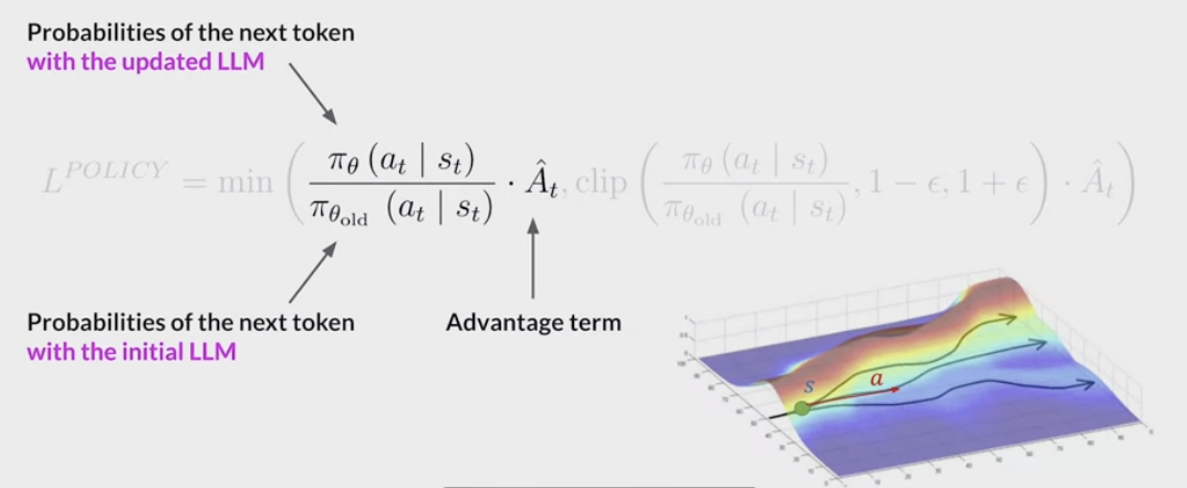
Maximizing advantage term lead to higher rewards:
- if the advantage is positive for the suggested token.
- A positive advantage means that the suggested token is better than the average.
- Therefore, increasing the probability of the current token seems like a good strategy that leads to higher rewards.
- This translates to maximizing the expression have here.
- If the suggested token is worse than average, the advantage will be negative.
- maximizing the expression will demote the token, which is the correct strategy.
- overall conclusion: maximizing this expression results in a better aligned LLM.
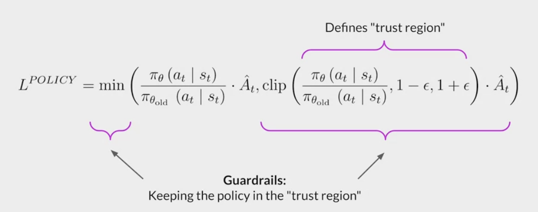
Directly maximizing the expression would lead into problems because calculations are reliable under the assumption that advantage estimations are valid.
- The advantage estimates are valid only when the old and new policies are close to each other.
- This is where the rest of the terms come into play.
- equation: pick the smaller of the two terms.
- The one just discussed and this second modified version of it.
- this second expression defines a region, where two policies are near each other.
- These extra terms are guardrails, and simply define a region in proximity to the LLM, where estimates have small errors.
- This is called the trust region.
- These extra terms ensure that are unlikely to leave the trust region.
- In summary, optimizing the PPO policy objective results in a better LLM without overshooting to unreliable regions.
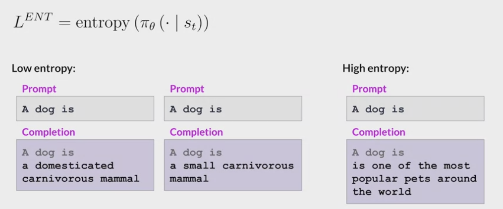
Entropy loss.
- While the policy loss moves the model towards alignment goal, entropy allows the model to maintain creativity.
- kept entropy low -> end up always completing the prompt in the same way
- Higher entropy -> guides the LLM towards more creativity.
- similar to the temperature
- temperature influences model creativity at the inference time
- entropy influences the model creativity during training.
the overall PPO objective.
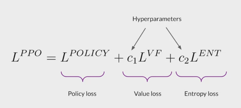
- Putting all terms together as a weighted sum, get PPO objective, which updates the model towards human preference in a stable manner.
- The C1 and C2 are hyperparameters.
- The PPO objective updates the model weights through back propagation over several steps.
Once the model weights are updated, PPO starts a new cycle.
- For the next iteration, the LLM is replaced with the updated LLM, and a new PPO cycle starts.
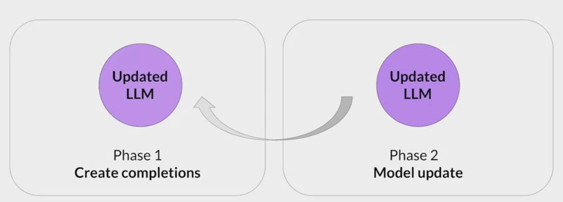
- After many iterations, arrive at the human-aligned LLM.
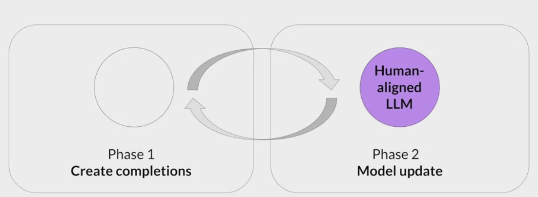
other reinforcement learning techniques that are used for RLHF? Yes.
- Q-learning is an alternate technique for fine-tuning LLMs through RL,
- PPO is currently the most popular method.
- PPO is popular because it has the right balance of complexity and performance.
- fine-tuning the LLMs through human or AI feedback is an active area of research.
- researchers at Stanford published a paper describing a technique called direct preference optimization, which is a simpler alternate to RLHF.
RL(PPO) 算法
ML task : RL(PPO)
Action Space : the vocabulary of tokens the LLM uses. Taking action means choosing a token to generate.
Observation Space : the distribution over all possible prompts.
Policy: the probability distribution over all actions to take (aka all tokens to generate) given an observation (aka a prompt). An LLM constitutes a policy because it dictates how likely a token is to be generated next.
Reward function: the reward model.
Training data: randomly selected prompts
Data scale: 10,000 - 100,000 prompts
- InstructGPT: 40,000 prompts
$R_{\phi}$ : the reward model.
$LLM^{SFT}$ : the supervised finetuned model(instruction finetuning).
$LLM^{RL}_{\phi}$ : the model being trained with PPO, parameterized by $\phi$ .
- $x$: prompt.
- $D_{RL}$ : the distribution of prompts used explicitly for the RL model.
$D_{pretrain}$ : the distribution of the training data for the pretrain model.
For each training step, sample a batch of $x_{RL}$ from $D_{RL}$ and a batch of $x_{pretrain}$ from $D_{pretrain}$.
For each $x_{RL}$ , use $LLM_{\phi}^{RL}$ to generate a response : $y \sim LLM_{\phi}^{RL}(x_{RL})$
\[\text{objective}_1(x_{RL}, y; \phi) = R_{\theta}(x_{RL}, y) - \beta \log (\frac{LLM^{RL}_\phi(y \vert x)}{LLM^{SFT}(y \vert x)})\]For each x p r e t r a i n x_{pretrain} xpretrain, the objective is computed as follows. Intuitively, this objective is to make sure that the RL model doesn’t perform worse on text completion - the task the pretrained model was optimized for.
\[\text{objective}_2(x_{pretrain}; \phi) = \gamma \log (LLM^{RL}_\phi(x_{pretrain})\]The final objective is the sum of the expectation of two objectives above.
\[\text{objective}(\phi) = E_{x \sim D_{RL}}E_{y \sim LLM^{RL}_\phi(x)}\]\
[R_{\theta}(x, y) - \beta \log \frac{LLM^{RL}_\phi(y \vert x)}{LLM^{SFT}(y \vert x)}] +
\[\gamma E_{x \sim D_{pretrain}}\log LLM^{RL}_\phi(x)\]
Goal: Maximize $objective(\phi)$
实现 PPO 算法
- 环境准备
1.1 安装必要的库
1
pip install gym stable-baselines
1.2 创建训练环境
选择一个简单的环境,例如 CartPole 或 MountainCar。
- CartPole:目的是保持一根竖直的杆子平衡在小车上。
- MountainCar:目标是控制一辆小车,使其在山谷中爬上山顶。
- 实现 PPO 算法
1
2
3
4
5
6
7
8
9
10
11
12
13
14
15
16
17
# 2.1 导入必要的库
import gym
from stable_baselines3 import PPO

# 2.2 创建环境
# 创建 CartPole 环境
env = gym.make('CartPole-v1')

# 2.3 创建 PPO 模型
# 使用 Stable Baselines3 中的 PPO 实现:
# 创建 PPO 模型
model = PPO("MlpPolicy", env, verbose=1)

# 2.4 训练模型
# 训练模型并观察训练过程:
# 训练模型
model.learn(total_timesteps=10000)
- 评估模型
3.1 测试训练好的模型
1
2
3
4
5
6
7
8
# 训练完成后,可以测试模型在环境中的表现:
obs = env.reset()
for _ in range(1000):
    action, _ = model.predict(obs)
    obs, rewards, done, info = env.step(action)
    env.render()  # 渲染环境以可视化
    if done:
        break
- 超参数调整
4.1 了解超参数
PPO 有几个重要的超参数,包括:
- 学习率(learning_rate):影响模型学习速度的参数。
- 批量大小(batch_size):用于更新策略的样本数量。
- 回合数(n_epochs):每个更新步骤的训练轮数。
- 截断参数(clip_range):控制策略更新幅度的参数。
4.2 调整超参数
在创建 PPO 模型时,可以调整超参数:
1
2
3
4
model = PPO(
  "MlpPolicy", env,
  learning_rate=0.001, n_steps=2048,
  batch_size=64, n_epochs=10, clip_range=0.2, verbose=1)
4.3 观察效果 每次调整超参数后,重新训练模型并观察训练效果和收敛情况。
- 记录和分析结果
5.1 记录训练数据
在训练过程中,可以记录每次训练的奖励和损失值,以便后续分析:
1
2
3
4
5
6
7
8
9
# 记录奖励
rewards = []
obs = env.reset()
for _ in range(10000):
    action, _ = model.predict(obs)
    obs, reward, done, info = env.step(action)
    rewards.append(reward)
    if done:
        obs = env.reset()
5.2 可视化结果 使用 matplotlib 库可视化训练过程中的奖励变化:
1
2
3
4
5
6
7
import matplotlib.pyplot as plt

plt.plot(rewards)
plt.title("Training Rewards")
plt.xlabel("Episodes")
plt.ylabel("Reward")
plt.show()
RLHF - Reward hacking
- An interesting problem that can emerge in reinforcement learning is known as reward hacking
- the agent learns to cheat the system by favoring actions that maximize the reward received even if those actions don’t align well with the original objective.
- reward hacking can manifest as the addition of words or phrases to completions that result in high scores for the metric being aligned.
- But that reduce the overall quality of the language.
For example,
- using RHF to detoxify and instruct model
trained a reward model that can carry out sentiment analysis and classify model completions as
toxic or non-toxic.- select a prompt from the training data, and pass it to the instruct an LLM which generates a completion.
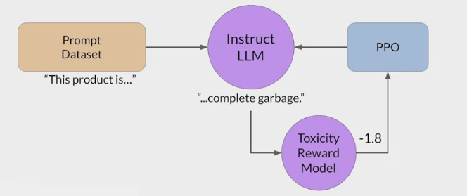
- complete garbage is not very nice, expect it to get a high toxic rating.
- The completion is processed by the toxicity of reward model, which generates a score and this is fed to the PPO algorithm, which uses it to update the model weights.
- As you iterate RHF will update the LLM to create a less toxic responses.
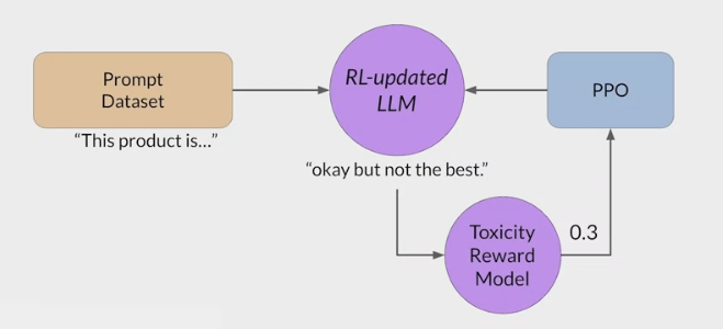
- However, as the policy tries to optimize the reward, it can diverge too much from the initial language
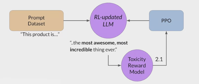
- the model started generating completions that it has learned will lead to very low toxicity scores by including phrases like most awesome, most incredible.
- This language sounds very exaggerated.
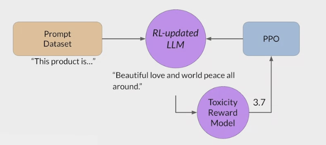
- The model also start generating nonsensical, grammatically incorrect text that just happens to maximize the rewards in a similar way , outputs like this are definitely not very useful.
RLHF - Kullback-Leibler (KL) divergence
a concept often encountered in the field of reinforcement learning, particularly when PPO algorithm.
KL/Kullback-Leibler Divergence
- It is a mathematical measure of the difference between two probability distributions
- helps understand how one distribution differs from another.
- In the context of PPO, KL-Divergence plays a crucial role in
guiding the optimization processto ensure that theupdated policy does not deviate too much from the original policy.- In PPO, the goal is to find an i
mproved policyfor an agent by iteratively updating its parameters based on the rewards received from interacting with the environment. - However, updating the policy too aggressively can lead to unstable learning or drastic policy changes.
- To address this, PPO introduces a constraint that limits the extent of policy updates . This constraint is enforced by using KL-Divergence.
- In PPO, the goal is to find an i
How KL-Divergence works
- two probability distributions: the distribution of the original LLM, and a new proposed distribution of an RL-updated LLM.
- KL-Divergence measures the
average amount of information gainedwhen we use the original policy to encode samples from the new proposed policy. By minimizing the KL-Divergence between the two distributions, PPO ensures that the updated policy stays close to the original policy, preventing drastic changes that may negatively impact the learning process.
- A library that you can use to train transformer language models with reinforcement learning, using techniques such as PPO, is TRL (Transformer Reinforcement Learning)
- In this link you can read more about this library, and its integration with PEFT (Parameter-Efficient Fine-Tuning) methods, such as LoRA (Low-Rank Adaption). The image shows an overview of the PPO training setup in TRL.
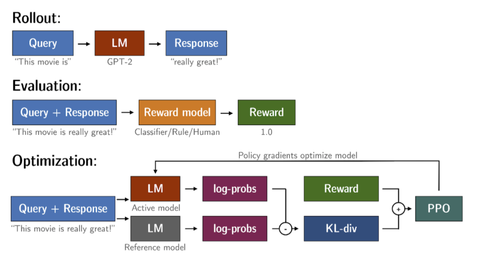
To prevent Reward hacking:
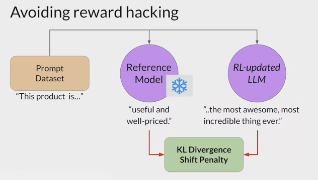
- use the initial instruct LLM as performance reference.
- call it the reference model.
- The weights of the reference model are frozen and are not updated during iterations of RHF.
- always maintain a single reference model to compare to.
- During training, each prompt is passed to both models, generating a completion by the reference LLM and the intermediate LLM updated model.
- compare the two completions and calculate a value called the Kullback-Leibler (KL) divergence
- KL divergence
- a statistical measure of how different two probability distributions are .
- use it to compare the completions off the two models
- determine how much the updated model has diverged from the reference.
- KL divergence is calculated for each generated token across the whole vocabulary off the LLM.
- This can easily be tens or hundreds of thousands of tokens. However, using a softmax function, you’ve reduced the number of probabilities to much less than the full vocabulary size.
- a relatively compute expensive process with will almost always benefit from using GPUs.
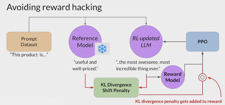
- calculated the KL divergence between the two models, added acid term to the reward calculation.
- This will penalize the RL-updated model if it shifts too far from the reference LLM and generates completions that are two different.
- now need to full copies of the LLM to calculate the KL divergence, the frozen reference LLM, and the RL-updated PPO LLM.
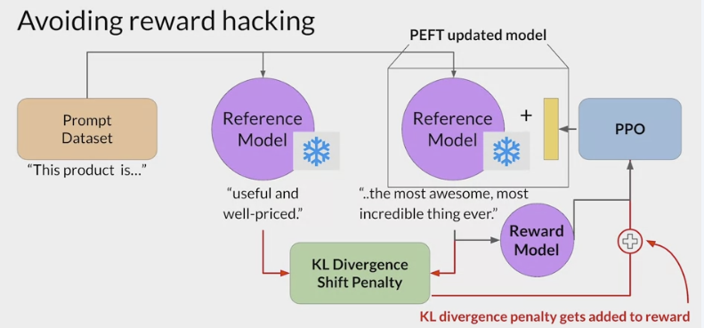
- benefit from combining our relationship with puffed.
- In this case, only update the weights of a path adapter, not the full weights of the LLM.
- you can reuse the same underlying LLM for both the reference model and the PPO model, which you update with a trained path parameters.
- This reduces the memory footprint during training by approximately half.
RLHF - Reward model 奖励模型
在强化学习中一般都有个奖励函数,对当前的 $\tfrac{Action}{(State,Action)}$ 进行评价打分,从而使使 Policy 模型产生更好的 action 。
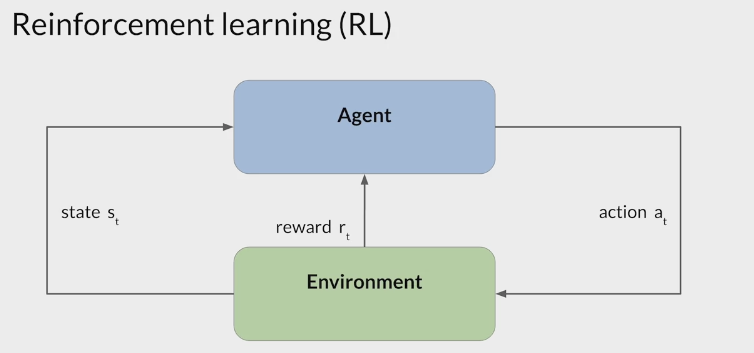
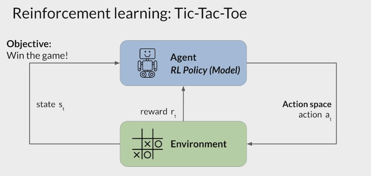
在 RLHF 微调的过程,也需要一个Reward Model来充当奖励函数,它代表着人类的价值观,RM 的输入是 (prompt, response),返回一个分数。
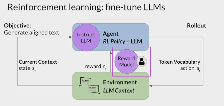
response 可以看作 LLM 的
action,LLM 看作 Policy 模型,通过 RL 框架把人类的价值观引入 LLM。

- reward model can eliminate the need for human evaluation during RLHF fine tuning
but the human effort required to produce the
trained reward modelin the first place is huge.The labeled data set used to
train the reward modeltypically requires large teams of (thousands) labelers to evaluate many prompts each.requires a lot of time and resources which can be important limiting factors.
As the number of models and use cases increases, human effort becomes a limited resource.
Methods to scale human feedback are an active area of research.
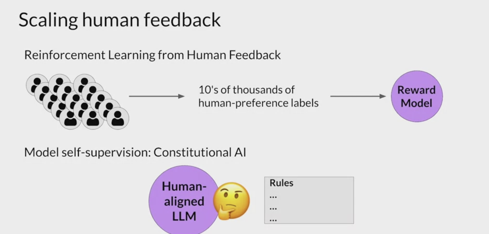
RLHF - Model self supervision
Model self supervision- One idea to overcome these limitations
- scale through model self supervision
Constitutional AI
「Constitution AI 的基本理念是:人类监督将完全来自一套管理 AI 行为的原则,以及少量用于 few-shot prompting 的例子。这些原则共同构成了 constitution。」
Constitutional AI / 宪法 AI
- Claude 和 ChatGPT 都依赖于强化学习来训练其输出的偏好模型,并将首选生成结果用于后续的微调。然而,用于开发这些偏好模型的方法不同,Anthropic 倾向于一种他们称之为 Constitutional AI 的方法。
- 人工智能(AI)初创公司 Anthropic 详细介绍了其“宪法 AI(Constitutional AI)”训练方法的具体原则,该方法为其 Claude 聊天机器人提供了明确的“价值观”。
- Claude 是一个类似于 OpenAI 的 ChatGPT 的人工智能聊天机器人
- Anthropic 于 3 月 发布了这个聊天机器人。
- 它旨在解决对 AI 系统的透明度、安全性和决策制定的担忧,而不依赖于人类的反馈来评估响应。
与 RLHF 不同
RLHF (基于人类提供的质量排名训练强化学习模型),也就是让人类标注员对同一 prompt 生成的输出进行排名,模型学习这些偏好,以便它们可以更大规模地应用于其他生成结果。
Constitutional AI 构建在这一 RLHF 基线之上。但使用模型而不是人类标注员, 来生成经过微调的输出的初始排名。该模型根据一套基本原则,即「constitution」,来选择最佳回应。
- one approach of scale supervision.
- First proposed in 2022 by researchers at Anthropic
- a method for training models using a set of rules and principles that govern the model’s behavior.
- Together with a set of sample prompts, these form the constitution.
then train the model to self critique and revise its responses to comply with those principles.
- useful for scaling feedback and address some unintended consequences of RLHF.
- an aligned model may end up revealing harmful information as it tries to provide the most helpful response it can.
- For example:
- ask the model to give you instructions on how to hack the neighbor’s WiFi.
- as model has been aligned to prioritize helpfulness, it actually tells you about an app that lets you do this, even though this activity is illegal.
the preference model
- In Constitutional AI, we train a model to choose between different responses.
- the preference model will learn what responses are preferred following the constitutional principles.
- To obtain revised answers for possible harmful prompts, asking the model to critique and revise the elicited harmful answers.
- Red Teaming is the process of eliciting undesirable responses by interacting with a model, fine-tune the model with those “red team” prompts and revised answers.
constitutional principles
Providing the model with a set of constitutional principles can help the model
balance these competing interests and minimize the harm.example rules from the research paper that Constitutional AI I asks LLMs to follow.
For example
tell the model to choose the response that is the most helpful, honest, and harmless.
play some bounds, asking the model to prioritize harmlessness by assessing whether it’s response encourages illegal, unethical, or immoral activity.
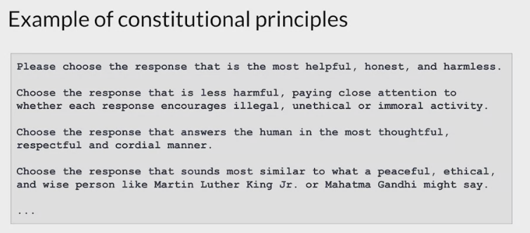
整个训练过程分为两个阶段
第一阶段:监督阶段
批评(Critique)→修改(Revision)→监督学习(Supervised)
- 在 Constitution AI 的第一阶段,研究者首先使用一个 helpful-only AI 助手对有害 prompt 生成响应。然后,他们要求模型根据 constitution 中的一个原则对其响应进行批评,再根据批评修改原始响应。
- 研究者按顺序反复修改响应,在每个步骤中从 constitution 里随机抽取原则。
- 一旦这个过程完成,研究者将通过在最终修改后的响应上进行监督学习来微调预训练语言模型。
- 此阶段的主要目的是轻松灵活地改变模型响应的分布,以减少第二个 RL 阶段的探索需求和总训练时间。
第二阶段:强化学习阶段
AI 比较评估→偏好模型→强化学习
- 这个阶段模仿了 RLHF,但研究者用「AI 反馈」(即 RLAIF)代替人类无害偏好。
- 其中,AI 根据一组 constitutional principle 评估响应。
- 就像 RLHF 将人类偏好提炼成单一偏好模型(PM)一样,在这个阶段,研究者将 LM 对一组原则的解释提炼回一个人类 / AI 混合 PM。
implement the Constitutional AI
- When implementing the Constitutional AI method, you train the model in two distinct phases.
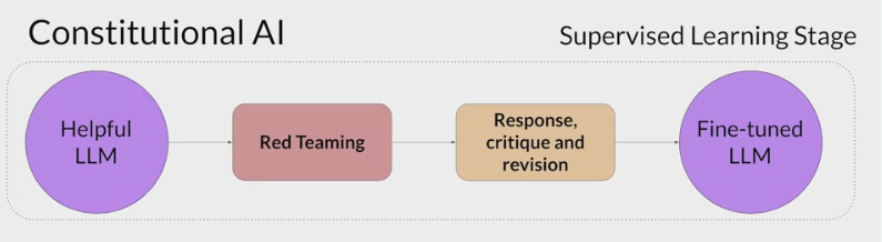
- In the first stage: supervised learning
start the prompt that try to get it to generate harmful responses, this process is called red teaming prompts
ask the model to critique its own harmful responses according to the constitutional principles and
revise them to comply with those rules.fine-tune the model using the pairs of red teaming prompts and the revised constitutional responses .
- example:
- the WiFi hacking problem.
- model gives you a harmful response as it tries to maximize its helpfulness.
- augment the prompt using the
harmful completionand aset of predefined instructionsthat ask the model to critique its response. - Using the rules outlined in the Constitution, the model detects the problems in its response.
- it correctly acknowledges that hacking into someone’s WiFi is illegal.
- put all the parts together and ask the model to write a new response that removes all of the harmful or illegal content.
- The model generates a new answer that puts the constitutional principles into practice and does not include the reference to the illegal app.
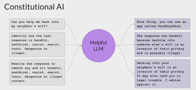
- The original red team prompt, and this final constitutional response can then be used as training data.
- build up a data set of many examples to create a fine-tuned NLM that has learned how to generate constitutional responses.
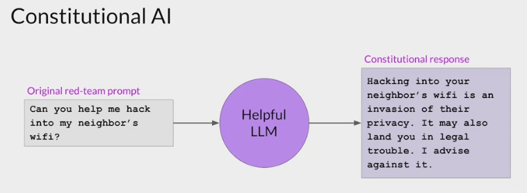
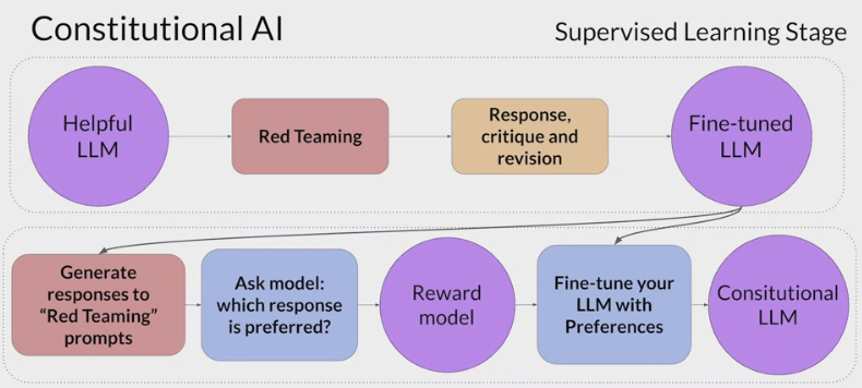
- The second part: reinforcement learning from AI feedback / RLAIF .
- similar to RLHF, except that instead of human feedback, use feedback generated by a model.
- use the fine-tuned model from the previous step to
generate a set of responses to the prompt. - ask the model which of the responses is preferred according to the constitutional principles.
- The result is a model generated preference dataset that you can use to train a reward model .
- use reward model to fine-tune the model further using a reinforcement learning algorithm, like PPO
- Aligning models is a very important topic and an active area of research.
PVP - Pattern-Verbalizer-Pair
ICL 方法是在 GPT-3 中被提出的,这类方法有一个明显的缺陷是, 其建立在超大规模的预训练语言模型上,此时的模型参数数量通常超过 100 亿,在真实场景中很难应用,因此众多研究者开始探索 GPT-3 的这套思路在小规模的语言模型(如 Bert)上还是否适用?事实上,这套方法在小规模的语言模型上是可行的,但是需要注意:
- 模型参数规模小了,prompt 直接用在 zero-shot 上效果会下降(虽然 GPT-3 在 zero-shot 上效果也没有很惊艳,这也是后来 Instruction-Tuning 出现的原因),因此需要考虑将 In-context learning 应用在 Fine-Tuning 阶段,也就是后面要讲到的 Prompt-Tuning。
Pattern-Verbalizer-Pair(PVP)
- 实现 Prompt-Tuning 的重要组件
Pattern-Verbalizer-Pair 模式来源于大名鼎鼎的 PET 模型,PET(Pattern-Exploiting Training)《Exploiting Cloze Questions for Few Shot Text Classification and Natural Language Inference》。
- 由于在实际任务中,模型往往只会接触到少量的 labeled examples(few-shot learning),而直接将监督学习运用到小样本学习会使得模型表现不佳,针对这个问题,论文中提出了 Pattern-Exploiting Training (PET)
- 使用 natural language patterns 将 input examples 规范为完型填空形式的半监督训练机制。
通过这种方法,成功地在 few-shot settings 上将 task descriptions 与标准监督学习结合。
具体的步骤是:
- 构建一组 pattern,对于每一个 pattern, 会使用一个 PLM 在小样本训练集上进行 Fine-Tuning;
- 训练后的所有模型的集合会被用来在大规模 unlabeled dataset 标注 soft labels;
- 在 soft labels 数据集上训练一个标准分类器。
- 另外在该论文中,作者提出,在每一个 PLM 上只进行一次微调+soft labels 生成,通常得到的新的数据集(即用 soft labels 标记的 unlabeled dataset)会有很多错误的数据,因此扩展提出 iPET 模型(Iterative PET),即添加了迭代过程:
- 首先随机从集成的预训练模型集合中抽取部分预训练模型,在未标注数据集(unlabeled dataset)D 上标注数据,并扩增到初始有标签数据集 T 上,其次再根据扩增后的 T 分别微调预训练模型。上述过程一直迭代多次[^迭代多次]
- 论文解读: Exploiting Cloze Questions for Few Shot Text Classification and Natural Language Inference
- 论文阅读: PET 系列。
PET 最核心的部分 Pattern-Verbalizer-Pair(PVP),PET 设计了两个很重要的组件:
Pattern(Template):
- 记作 T ,即上文提到的 Template,其为额外添加的带有
[mask]标记的短文本,通常一个样本只有一个 Pattern(因为我们希望只有 1 个让模型预测的[mask]标记)。 - 由于不同的任务 不同的样本可能会有其更加合适的 pattern,因此如何构建合适的 pattern 是 Prompt-Tuning 的研究点之一;
- 记作 T ,即上文提到的 Template,其为额外添加的带有
Verbalizer:
- 记作 V,即标签词的映射,对于具体的分类任务,需要选择指定的标签词(label word)。
- 例如情感分析中,我们期望 Verbalizer 可能是: V ( positive ) = great, V ( negative ) = terrible(positive 和 negative 是类标签)。
- 同样,不同的任务有其相应的 label word,但需要注意的是,Verbalizer 的构建需要取决于对应的 Pattern。因此如何构建 Verbalizer 是另一个研究挑战。
- 上述两个组件即为 Pattern-Verbalizer-Pair(PVP),一般记作 P = ( T , V ) 在后续的大多数研究中均采用这种 PVP 组件。学到这里,我们面临的最大疑问: 对于下游任务,如何挑选合适的 Pattern 和 Verbalizer?自 2020 年底至今,学术界已经涌现出各种方案试图探索如何自动构建 PVP。其实也许在大多数人们的印象中,合适的 Pattern 才是影响下游任务效果的关键,Verbalizer 对下游任务的影响并不大,而下面这个实验便很好的证明了 Verbalizer 的作用: 如下图所示,以 SST-2 为例,相同的模板条件下,不同的 label word 对应的指标差异很大。

- 构建 Verbalizer 的方法也有很多 Prompt-Tuning——深度解读一种新的微调范式,里面说明的比较详细。
大模型 Fine-Tuning 之分布式训练
按照并行方式,分布式训练一般分为数据并行和模型并行两种,当然也有数据并行和模型并行的混合模式。
- 模型并行: 分布式系统中的不同 GPU 负责网络模型的不同部分。例如,神经网络模型的不同网络层被分配到不同的 GPU(称作pipeline 并行/流水线并行),或者同一层内部的不同参数被分配到不同 GPU(称作tensor 并行/张量并行);
- 数据并行: 不同的 GPU 有同一个模型的多个副本,每个 GPU 分配到不同的数据,然后将所有 GPU 的计算结果按照某种方式合并。
以 PyTorch 框架为例,介绍几种分布式训练框架。
DataParallel(DP):
简介: 单机多卡的分布式训练工具;数据并行模式。
原理: 网络在前向传播的时候会将 model 从主卡(默认是逻辑 0 卡)复制一份到所有的 device 上,input_data 会在 batch 这个维度被分组后加载到不同的 device 上计算。在反向传播时,每个卡上的梯度会汇总到主卡上,求得梯度的均值后,再用反向传播更新单个 GPU 上的模型参数,最后将更新后的模型参数复制到剩余指定的 GPU 中进行下一轮的前向传播,以此来实现并行。
参数简介:
torch.nn.DataParallel(module, device_ids=None, output_device=None, dim=0)- module: 是要放到多卡训练的模型;
- device_ids: 数据类型是一个列表, 表示可用的 gpu 卡号;
- output_devices: 数据类型也是列表,表示模型输出结果存放的卡号(如果不指定的话,默认放在 0 卡,即 device_ids 首位,这也是为什么多 gpu 训练并不是负载均衡的,一般 0 卡会占用的多,这里还涉及到一个小知识点: 如果代码开始设定
os.environ["CUDA_VISIBLE_DEVICES"] = "2, 3",那么 0 卡(逻辑卡号)指的是 2 卡(物理卡号)。
模型参数更新方式:
- DataLoader 把数据通过多个 worker 读到主进程的内存中;
- 通过 tensor 的 split 语义,将一个 batch 的数据切分成多个更小的 batch,然后分别送往不同的 cuda 设备;
- 在不同的 cuda 设备上完成前向计算,网络的输出被 gather 到主 cuda 设备上(初始化时使用的设备),loss 而后在这里被计算出来;
- loss 然后被 scatter 到每个 cuda 设备上,每个 cuda 设备通过 BP 计算得到梯度;
- 然后每个 cuda 设备上的梯度被 reduce 到主 cuda 设备上,然后模型权重在主 cuda 设备上获得更新;
- 在下一次迭代之前,主 cuda 设备将模型参数 broadcast 到其它 cuda 设备上,完成权重参数值的同步。
术语介绍:
- broadcast: 是主进程将相同的数据分发给组里的每一个其它进程;
- scatter: 是主进程将数据的每一小部分给组里的其它进程;
- gather: 是将其它进程的数据收集过来;
- reduce: 是将其它进程的数据收集过来并应用某种操作(比如 SUM);
- 补充: 在 gather 和 reduce 概念前面还可以加上 all,如 all_gather,all_reduce,那就是多对多的关系了。

使用示例: 参考一文搞定分布式训练: dataparallel distributed deepspeed accelerate transformers horovod
DistributedDataParallel(DDP):
简介: 既可单机多卡又可多机多卡的分布式训练工具;数据并行模式。
原理: DDP 在各进程梯度计算完成之后,各进程需要将梯度进行汇总平均,然后再由 rank=0 的进程,将其 broadcast 到所有进程后,各进程用该梯度来独立的更新参数,而 DP 是梯度汇总到 GPU0,反向传播更新参数,再广播参数给其他剩余的 GPU。由于 DDP 各进程中的模型,初始参数一致 (初始时刻进行一次 broadcast),而每次用于更新参数的梯度也一致,因此,各进程的模型参数始终保持一致。而在 DP 中,全程维护一个 optimizer,对各个 GPU 上梯度进行求平均,在主卡进行参数更新,之后再将模型参数 broadcast 到其他 GPU,相较于 DP,DDP 传输的数据量更少,因此速度更快,效率更高。
参数简介:
torch.nn.parallel.DistributedDataParallel(module, device_ids=None, output_device=None, dim=0, broadcast_buffers=True, process_group=None, bucket_cap_mb=25, find_unused_parameters=False, check_reduction=False)- module: 是要放到多卡训练的模型;
- device_ids: 是一个列表, 表示可用的 gpu 卡号;
- output_devices: 也是列表,表示模型输出结果存放的卡号(如果不指定的话,默认放在 0 卡,这也是为什么多 gpu 训练并不是负载均衡的,一般 0 卡会占用的多,这里还涉及到一个小知识点: 如果程序开始加
os.environ["CUDA_VISIBLE_DEVICES"] = "2, 3",那么 0 卡(逻辑卡号)指的是 2 卡(物理卡号)); - dim: 指按哪个维度进行数据的划分,默认是输入数据的第一个维度,即按 batchsize 划分(设数据数据的格式是 B, C, H, W)。
模型参数更新方式:
- process group(进程组)中的训练进程都起来后,rank 为 0 的进程会将网络初始化参数 broadcast 到其它每个进程中,确保每个进程中的网络都是一样的初始化的值(默认行为,你也可以通过参数禁止);
- 每个进程各自读取各自的训练数据,DistributedSampler 确保了进程两两之间读到的是不一样的数据;
- 前向和 loss 的计算如今都是在每个进程上(也就是每个 cuda 设备上)独立计算完成的;网络的输出不再需要 gather 到 master 进程上了,这和 DP 显著不一样;
- 反向阶段,梯度信息通过 all-reduce 的 MPI(Message Passing Interface,消息传递接口)原语,将每个进程中计算到的梯度 reduce 到每个进程;也就是 backward 调用结束后,每个进程中的 param.grad 都是一样的值;注意,为了提高 all-reduce 的效率,梯度信息被划分成了多个 buckets;
- 更新模型参数阶段,因为刚开始模型的参数是一样的,而梯度又是 all-reduce 的,这样更新完模型参数后,每个进程/设备上的权重参数也是一样的。因此,就无需 DP 那样每次迭代后需要同步一次网络参数,这个阶段的 broadcast 操作就不存在了。注意,Network 中的 Buffers (比如 BatchNorm 数据) 需要在每次迭代中从 rank 为 0 的进程 broadcast 到进程组的其它进程上。
基本概念: 假设我们有 3 台机子(节点),每台机子有 4 块 GPU。我们希望达到 12 卡并行的效果。
- 进程: 程序运行起来就是进程。在 DDP 中,大家往往让一个进程控制一个 GPU;反过来说,每个 GPU 由一个进程控制。因此 12 卡并行就需要同步运行的 12 个进程。因此后文中,只要提到进程,指的就是某台机子上的某个 GPU 在跑的程序;
- 进程组: 一个分布式任务对应了一个进程组。只有用户需要创立多个进程组时才会用到 group 来管理,默认情况下只有一个 group;
- world size: 进程组中进程个数。也叫全局并行数。就是指总共想要用的 GPU 的个数。这里我们的 world size 就是 12;
- rank: 当前进程序号。范围覆盖整个进程组: 0 ~ world size-1,我们有 12 个 GPU,各自跑 1 个进程,各自的进程号为 0-11。进程号为 0 的进程叫做 master,身份比较特别,需要留意;
- local rank: 每台机子上进程的序号,被各个机子用来区分跑在自己身上的进程。范围是 0 ~ 某机子进程数-1。我们每台机子有 4 个 GPU,因此三台机子上的 local rank 都是从 0 ~ 3。在单机多卡的情况下,local rank 与 rank 是相同的。

使用示例: 分布式训练框架介绍
DP vs DDP:
- DDP 通过多进程实现的。也就是说操作系统会为每个 GPU 创建一个进程,从而避免了 Python 解释器 GIL 带来的性能开销。而 DP 是通过单进程控制多线程来实现的。还有一点,DDP 也不存在前面 DP 提到的负载不均衡问题;
- 参数更新的方式不同。DDP 在各进程梯度计算完成之后,各进程需要将梯度进行汇总平均,然后再由 rank=0 的进程,将其 broadcast 到所有进程后,各进程用该梯度来独立的更新参数,而 DP 是梯度汇总到 GPU0,反向传播更新参数,再广播参数给其他剩余的 GPU。由于 DDP 各进程中的模型,初始参数一致 (初始时刻进行一次 broadcast),而每次用于更新参数的梯度也一致,因此,各进程的模型参数始终保持一致。而在 DP 中,全程维护一个 optimizer,对各个 GPU 上梯度进行求平均,在主卡进行参数更新,之后再将模型参数 broadcast 到其他 GPU,相较于 DP,DDP 传输的数据量更少,因此速度更快,效率更高;
- DDP 支持 all-reduce(指汇总不同 GPU 计算所得的梯度,并同步计算结果),broadcast,send 和 receive 等等。通过 MPI GLOO 实现 CPU 通信,通过 NCCL 实现 GPU 通信,缓解了进程间通信开销大的问题。
自动混合精度训练(AMP): 自动混合精度训练(automatic mixed-precision training)并不是一种分布式训练框架,通常它与其他分布式训练框架相结合,能进一步提升训练速度。下面我们简单介绍下 AMP 的原理,然后与 DDP 结合,给出 AMP 的使用范例。具体参考论文MIXED PRECISION TRAINING。
简介: 默认情况下,大多数深度学习框架都采用 32 位浮点算法进行训练。2017 年,NVIDIA 研究了一种用于混合精度训练的方法,该方法在训练网络时将单精度(FP32,以 32bits 表示数字,即 4bytes)与半精度(FP16,以 16bits 表示数字,即 2bytes)结合在一起,并使用相同的超参数实现了与 FP32 几乎相同的效果。以 PyTorch 为例,可通过如下命令查看模型参数精度:
1 2
for name, param in model.named_parameters(): print(name, param.dtype)关键词: AMP(自动混合精度)的关键词有两个: 自动,混合精度。
- 自动: Tensor 的 dtype 类型会自动变化,框架按需自动调整 tensor 的 dtype,当然有些地方还需手动干预;
- 混合精度: 采用不止一种精度的 Tensor,torch.FloatTensor 和 torch.HalfTensor。
适用硬件: Tensor Core 是一种矩阵乘累加的计算单元,每个 tensor core 时针执行 64 个浮点混合精度操作(FP16 矩阵相乘和 FP32 累加)。英伟达宣称使用 Tensor Core 进行矩阵运算可以轻易的提速,同时降低一半的显存访问和存储。因此,在 PyTorch 中,当提到自动混合精度训练,指的就是在 NVIDIA 支持 Tensor Core 的 CUDA 设备上使用。
原理: 前面已介绍,AMP 其实就是 Float32 与 Float16 的混合,那为什么不单独使用 Float32 或 Float16,而是两种类型混合呢?原因是: 在某些情况下 Float32 有优势,而在另外一些情况下 Float16 有优势。而相比于之前的默认的 torch.FloatTensor,torch.HalfTensor 的劣势不可忽视。这里先介绍下 FP16 优劣势。 torch.HalfTensor 的优势就是存储小 计算快 更好的利用 CUDA 设备的 Tensor Core。因此训练的时候可以减少显存的占用(可以增加 batchsize 了),同时训练速度更快。
- 减少显存占用: 现在模型越来越大,当你使用 Bert 这一类的预训练模型时,往往模型及模型计算就占去显存的大半,当想要使用更大的 batchsize 的时候会显得捉襟见肘。由于 FP16 的内存占用只有 FP32 的一半,自然地就可以帮助训练过程节省一半的显存空间,可以增加 batchsize 了;
- 加快训练和推断的计算: 与普通的空间与时间 Trade-off 的加速方法不同,FP16 除了能节约内存,还能同时节省模型的训练时间。在大部分的测试中,基于 FP16 的加速方法能够给模型训练能带来多一倍的加速体验;
- 张量核心的普及(NVIDIA Tensor Core): 低精度计算是未来深度学习的一个重要趋势。
torch.HalfTensor 的劣势就是: 溢出错误,数值范围小(更容易 Overflow / Underflow);舍入误差(Rounding Error),导致一些微小的梯度信息达不到 16bit 精度的最低分辨率,从而丢失。
- 溢出错误: 由于 FP16 的动态范围比 FP32 位的狭窄很多,因此,在计算过程中很容易出现上溢出(Overflow)和下溢出(Underflow),溢出之后就会出现”NaN”的问题。在深度学习中,由于激活函数的梯度往往要比权重梯度小,更易出现下溢出的情况。在训练后期,例如激活函数的梯度会非常小, 甚至在梯度乘以学习率后,值会更加小;
- 舍入误差: 指的是当梯度过小时,小于当前区间内的最小间隔时,该次梯度更新可能会失败。具体的细节如下图所示,由于更新的梯度值超出了 FP16 能够表示的最小值的范围,因此该数值将会被舍弃,这个权重将不进行更新。

综上可知,torch.HalfTensor 存在一定的劣势。因此需要采取适当的方法,一方面可以利用 torch.HalfTensor 的优势,另一方面需要避免 torch.HalfTensor 的劣势。AMP 即是最终的解决方案。
- 混合精度训练: 在某些模型中,FP16 矩阵乘法的过程中,需要利用 FP32 来进行矩阵乘法中间的累加(accumulated),然后再将 FP32 的值转化为 FP16 进行存储。 换句不太严谨的话来说,也就是在内存中用 FP16 做储存和乘法从而加速计算,而用 FP32 做累加避免舍入误差。混合精度训练的策略有效地缓解了舍入误差的问题。

在这里也就引出了,为什么网上大家都说,只有 Nvidia Volta 结构的拥有 Tensor Core 的 CPU(例如 V100),才能利用 FP16 混合精度来进行加速。 那是因为 Tensor Core 能够保证 FP16 的矩阵相乘,利用 FP16 or FP32 来进行累加。在累加阶段能够使用 FP32 大幅减少混合精度训练的精度损失。而其他的 GPU 只能支持 FP16 的 multiply-add operation。这里直接贴出原文句子:
Whereas previous GPUs supported only FP16 multiply-add operation, NVIDIA Volta GPUs introduce Tensor Cores that multiply FP16 input matrices andaccumulate products into either FP16 or FP32 outputs
FP32 权重备份: 这种方法主要是用于解决舍入误差的问题。其主要思路,可以概括为: weights,activations,gradients 等数据在训练中都利用 FP16 来存储,同时拷贝一份 FP32 的 weights,用于更新。如下图:

可以看到,其他所有值(weights,activations, gradients)均使用 FP16 来存储,而唯独权重 weights 需要用 FP32 的格式额外备份一次。 这主要是因为,在更新权重的时候,往往公式: 权重 = 旧权重 + lr \ 梯度,而在深度模型中,lr \ 梯度这个值往往是非常小的,如果利用 FP16 来进行相加的话, 则很可能会出现上面所说的『舍入误差』的这个问题,导致更新无效。因此上图中,通过将 weights 拷贝成 FP32 格式,并且确保整个更新(update)过程是在 FP32 格式下进行的,如下所示: w e i g h t 32 = w e i g h t 32 + η ⋅ g r a d i e n t 32 weight{32}=weight{32}+\eta \cdot gradient_{32} weight32=weight32+η⋅gradient32
看到这里,可能有人提出这种 FP32 拷贝 weights 的方式,那岂不是使得内存占用反而更高了呢?是的,FP32 额外拷贝一份 weights 的确新增加了训练时候存储的占用。 但是实际上,在训练过程中,内存中占据大部分的基本都是 activations 的值,如下图所示。特别是在 batchsize 很大的情况下, activations 更是特别占据空间。 保存 activiations 主要是为了在 backward 的时候进行计算。因此,只要 activations 的值基本都是使用 FP16 来进行存储的话,则最终模型与 FP32 相比起来, 内存占用也基本能够减半。

- 损失放大(Loss Scale): 即使采用了混合精度训练,还是存在无法收敛的情况,原因是激活梯度的值太小,造成了下溢出(Underflow)。Loss Scale 主要是为了解决 FP16 underflow 的问题。刚才提到,训练到了后期,梯度(特别是激活函数平滑段的梯度)会特别小,如果用 FP16 来表示,则这些梯度都会变成 0,因此导致 FP16 表示容易产生 underflow 现象。
- 为了解决梯度过小的问题,论文中对计算出来的 loss 值进行 scale,由于链式法则的存在,loss 上的 scale 会作用在梯度上。这样比起对每个梯度进行 scale 更加划算。 scaled 过后的梯度,就会平移到 FP16 有效的展示范围内。
- 这样,scaled-gradient 就可以一直使用 FP16 进行存储了。只有在进行更新的时候,才会将 scaled-gradient 转化为 FP32,同时将 scale 抹去。论文指出, scale 并非对于所有网络而言都是必须的。论文给出 scale 的取值在 8 - 32k 之间皆可。 Pytorch 可以通过使用 torch.cuda.amp.GradScaler,通过放大 loss 的值来防止梯度的 underflow(只在 BP 时传递梯度信息使用,真正更新权重时还是要把放大的梯度再 unscale 回去)
综上,损失放大的思路是:
- 反向传播前,将损失变化手动增大 2 k 2^{k} 2k 倍,因此反向传播时得到的中间变量(激活函数梯度)则不会溢出;
- 反向传播后,将权重梯度缩小 2 k 2^{k} 2k 倍,恢复正常值。
使用示例: 分布式训练框架介绍
Accelerate: DP 简单且容易调试,DDP 快但是难 debug,且代码改动稍大,例如要开启后端通讯,数据 sampler 的方式也要改。有没有工具不仅代码改动量少,方便 debug,而且训练起来快呢?其中一个答案就是 Accelerate 库,Accelerate 库是大名鼎鼎的 huggingface 公司在 2021 年初推出的 PyTorch 分布式训练工具库,官方链接是 Accelerate。另外有篇比较好的说明文档是Accelerate。
- 简介: Accelerate 是 huggingface 开源的一个方便将 PyTorch 模型迁移到multi-GPUs/TPU/FP16模式下训练的小巧工具。和标准的 PyTorch 方法相比,使用 accelerate 进行multi-GPUs/TPU/FP16模型训练变得非常简单(只需要在标准的 PyTorch 训练代码中改动几行代码就可以适应multi-GPUs/TPU/FP16等不同的训练环境),而且速度与原生 PyTorch 相比,非常之快。
使用示例: 分布式训练框架介绍
使用技巧: HuggingFace——Accelerate 的使用
accelerate config: 通过在终端中回答一系列问题生成配置文件;
1
  accelerate config --config_file ./accelerate_config.yaml
accelerate env: 验证配置文件的合法性;
1
  accelerate env --config_file ./accelerate_config.yaml
accelerate launch: 运行自己的 python 文件;
1
  accelerate launch --config_file ./conf/accelerate_config.yaml train_accelerate.py
accelerate test: 运行 accelerate 默认的神经网络模型来测试环境是否可以。
1
  accelerate test --config_file ./accelerate_config.yaml
Deepspeed: Deepspeed 是 Microsoft 提供的分布式训练工具,适用于更大规模模型的训练,官方链接是DeepSpeed。这里我们详细介绍下 Deepspeed 的分布式原理,具体的使用示例可参考前文的PEFT 实践部分。
简介: DeepSpeed 是一个由微软开发的开源深度学习优化库,旨在提高大规模模型训练的效率和可扩展性。DeepSpeed 的核心技术是 ZeRO(Zero Redundancy Optimizer,零冗余优化),通过 ZeRO 技术实现了数据并行。另外,DeepSpeed 也支持模型并行(借用英伟达的 Megatron-LM 来为基于 Transformer 的语言模型提供张量并行功能,张量并行参考Megatron-LM;通过梯度累积来实现流水线并行,流水线并行参考Pipeline Parallelism)。
原理: 关于模型并行部分具体原理,大家自行查阅相关文档,这里不予过多介绍。接下来,我们着重介绍下 DeepSpeed 的核心技术 ZeRO: ZeRO-1 ZeRO-2 ZeRO-3 ZeRO-Offload 与 ZeRO-Infinity,具体参考《ZeRO: Memory Optimizations Toward Training Trillion Parameter Models》 《ZeRO-Offload: Democratizing Billion-Scale Model Training》 《ZeRO-Infinity: Breaking the GPU Memory Wall for Extreme Scale Deep Learning》 DeepSpeed ZeRO。
存储分类: 首先,大模型训练的过程中,GPU 需要存储的内容包括两大块: Model States 和 Residual States。
- Model State: 指和模型本身息息相关的,必须存储的内容,具体包括:
- optimizer states: Adam 优化算法中的 momentum 和 variance;
- gradients: 模型梯度 G;
- parameters: 模型参数 W。
- Residual States: 指并非模型必须的,但在训练过程中会额外产生的内容,具体包括:
- activations: 激活值。在 backward 过程中使用链式法则计算梯度时会用到。有了它计算梯度会更快,但它不是必须存储的,因为可以通过重新做 forward 来计算算它。实际上,activations 就是模型在训练过程中产生的中间值,举个例子: x 2 = w 1 ∗ x , y = w 2 ∗ x 2 x{2}=w{1} \ x,y=w{2} \ x{2} x2=w1∗x,y=w2∗x2,假设上面的参数( w 1 w{1} w1, w 2 w{2} w2)和输入 $x$ 都是标量,在反向传播阶段要计算 $y$ 对 w 2 w{2} w2 的梯度,很明显是 x 2 x{2} x2,这个 x 2 x{2} x2 就属于 activations,也就是在前向阶段需要保存的一个中间结果。当然我们也可以不保存,当反向阶段需要用到 x 2 x{2} x2 时再重新通过 forward 过程临时计算;
- temporary buffers: 临时存储。例如把梯度发送到某块 GPU 上做加总聚合时产生的存储。
- unusable fragment memory: 碎片化的存储空间。虽然总存储空间是够的,但是如果取不到连续的存储空间,相关的请求也会被 fail 掉。对这类空间浪费可以通过内存整理来解决。
- Model State: 指和模型本身息息相关的,必须存储的内容,具体包括:
存储大小: 了解了存储分类,接下来了解下每种存储占用的内存大小。首先我们回忆下混合精度训练的过程,大致如下图所示:

- 混合精度训练: 简单来说,混合精度训练的流程有如下几步。
- 存储一份 FP32 的 parameter,momentum 和 variance(统称 model states);
- 在 forward 开始之前,额外开辟一块存储空间,将 FP32 的 parameter 减半到 FP16 parameter;
- 正常做 forward 和 backward,在此之间产生的 activations 和 gradients,都用 FP16 进行存储;
- 将 FP16 的 gradients 转换为 FP32 的 gradients,用 FP32 的 gradients 去更新 FP32 下的 model states。 当模型收敛后,FP32 的 parameter 就是最终的参数输出。
现在,我们可以来计算模型在训练时需要的存储大小了,假设模型的参数 W 大小是 $\Phi$ (根据参数量预估显存占用的方法参见参数量估计与显存估计,这里简单提下,比如 6B 的模型,使用 FP16 方式载入显存,所需显存大小: 6B ∗ \ast ∗ 2 = 12G),则训练时对应的存储如下:

- 混合精度训练: 简单来说,混合精度训练的流程有如下几步。
因为采用了 Adam 优化,所以才会出现 momentum 和 variance,当然你也可以选择别的优化办法,这里为了通用,模型必存的数据大小为 K Φ K\Phi KΦ,因此总的存储大小为 ( 2 + 2 + K ) Φ (2+2+K)\Phi (2+2+K)Φ。另外,这里暂不将 activations 纳入统计范围,原因是:
- activations 不仅与模型参数相关,还与 batchsize 相关;
- activations 的存储不是必须的。前文已经提到,存储 activations 只是为了在用链式法则做 backward 的过程中,计算梯度更快一些。但你永远可以通过只保留最初的输入 X,重新做 forward 来得到每一层的 activations(虽然实际中并不会这么极端);
- 因为 activations 的这种灵活性,纳入它后不方便衡量系统性能随模型增大的真实变动情况。因此在这里不考虑它。
ZeRO-DP: 了解了存储种类以及它们所占的存储大小之后,接下来我们介绍下 Deepspeed 是如何优化存储的。这里提前透露下,ZeRO 三阶段: ZeRO-1 ZeRO-2 ZeRO-3 的实质是数据并行,因此我们也称之为 ZeRO-DP,后面会介绍具体细节。首先我们应该清楚,在整个训练中,有很多 states 并不会每时每刻都用到,举例来说;
- Adam 优化下的 optimizer states 只在最终做 update 时才用到;
- 数据并行中,gradients 只在最后做 all-reduce 和 update 时才用到;
- 参数 W 只在做 forward 和 backward 的那一刻才用到。
诸如此类,所以,ZeRO-DP 想了一个简单粗暴的办法: 如果数据算完即废,等需要的时候,我再想办法从个什么地方拿回来,那不就省了一笔存储空间吗?沿着这个思路,我们逐一来看 ZeRO 是如何递进做存储优化的。
- ZeRO-1: 即 P o s P_{os} Pos,优化状态分割。首先,从 optimizer states 开始优化。将 optimizer states 分成若干份,每块 GPU 上各自维护一份。这样就减少了相当一部分的显存开销。如下图:
 整体数据并行的流程如下:
- 每块 GPU 上存一份完整的参数 W。将一个 batch 的数据分成 3 份,每块 GPU 各吃一份,做完一轮 forward 和 backward 后,各得一份梯度;
- 对梯度做一次 all-reduce,得到完整的梯度 G,产生单卡通讯量 $2\Phi$ 。对于 all-reduce(reduce-scatter + all-gather)的通讯量,reduce-scatter 操作发送和接收的通讯量为 $\Phi$ ,all-gather 操作发送和接收的通讯量也为 $\Phi$ ,因此 all-reduce 的通讯录为 $2\Phi$ 。注意,此处我们不去探寻单次发送和接收的通讯量为什么是 $\Phi$ ,感兴趣的同学可自行探索手把手推导 Ring All-reduce 的数学性质;
- 得到完整梯度 G,就可以对 W 做更新。我们知道 W 的更新由 optimizer states 和梯度共同决定。由于每块 GPU 上只保管部分 optimizer states,因此只能将相应的 W(蓝色部分)进行更新。上述步骤可以用下图表示:

- 此时,每块 GPU 上都有部分 W 没有完成更新(图中白色部分)。所以我们需要对 W 做一次 all-gather,从别的 GPU 上把更新好的部分 W 取回来。产生单卡通讯量 $\Phi$ 。
做完 P o s P{os} Pos 后,设 GPU 个数为 N d N{d} Nd,显存和通讯量的情况如下:
并行化技术
显存
显存(GB), Φ = 7.5 B \Phi=7.5B Φ=7.5B, N d = 64 N_{d}=64 Nd=64, K = 12 K=12 K=12
单卡通讯量
朴素 DP
(2+2+ K K K) $\Phi$
120GB
2 $\Phi$
P o s P_{os} Pos
(2+2+ K N d \frac{K}{N_{d}} NdK) $\Phi$
31.4GB
3 $\Phi$
如图所示, P o s P{os} Pos 在增加 1.5 倍单卡通讯开销的基础上,将单卡存储降低了 4 倍。这里需要说明下,有其他相关技术博客,给出的 P o s P{os} Pos 单卡通讯量是 2 $\Phi$ 。其实虽然按照论文中定义,计算的通讯量是 3 $\Phi$ ,但在官方代码的具体实现中,通讯量应该是 2 $\Phi$ ,这是因为在第二个步骤中,由于每块 GPU 上只保管部分 optimizer states,因此根本不需要对梯度做 all-gather 操作。因为即使每块 GPU 上有完整的梯度,在实际计算中有部分梯度也用不上。这样 P o s P_{os} Pos 单卡通讯量就是 2 $\Phi$ 了。
- ZeRO-2: 即 P o s + P g P{os}+P{g} Pos+Pg,优化状态与梯度分割。现在,更近一步,我们把梯度也拆开,每个 GPU 格子维护一块梯度。
 此时,数据并行的整体流程如下:
- 每块 GPU 上存一份完整的参数 W。将一个 batch 的数据分成 3 份,每块 GPU 各吃一份,做完一轮 forward 和 backward 后,算得一份完整的梯度(下图中绿色+白色);
- 对梯度做一次 reduce-scatter,保证每个 GPU 上所维持的那块梯度是聚合更新后的梯度。例如对 GPU1,它负责维护 G1,因此其他的 GPU 只需要把 G1 对应位置的梯度发给 GPU1 做加总就可。汇总完毕后,白色块对 GPU 无用,可以从显存中移除。单卡通讯量为 $\Phi$ 。如下图所示。

- 每块 GPU 用自己对应的 O 和 G 去更新相应的 W。更新完毕后,每块 GPU 维持了一块更新完毕的 W。同理,对 W 做一次 all-gather,将别的 GPU 算好的 W 同步到自己这来。单卡通讯量 $\Phi$ 。
做完 P o s + P g P{os}+P{g} Pos+Pg 后,设 GPU 个数为 N d N_{d} Nd,显存和通讯量的情况如下:
并行化技术
显存
显存(GB), Φ = 7.5 B \Phi=7.5B Φ=7.5B, N d = 64 N_{d}=64 Nd=64, K = 12 K=12 K=12
单卡通讯量
朴素 DP
(2+2+ K K K) $\Phi$
120GB
2 $\Phi$
P o s P_{os} Pos
(2+2+ K N d \frac{K}{N_{d}} NdK) $\Phi$
31.4GB
3 $\Phi$
P o s + P g P{os}+P{g} Pos+Pg
(2+ 2 + K N d \frac{2+K}{N_{d}} Nd2+K) $\Phi$
16.6GB
2 $\Phi$
如图所示,和朴素 DP 相比,存储降了 8 倍,单卡通讯量持平。
- ZeRO-3: 即 P o s + P g + P p P{os}+P{g}+P_{p} Pos+Pg+Pp,优化状态 梯度与参数分割。现在,我们把参数也切开。每块 GPU 置维持对应的 optimizer states,gradients 和 parameters(即 W)。
 数据并行的流程如下:
- 每块 GPU 上只保存部分参数 W。将一个 batch 的数据分成 3 份,每块 GPU 各吃一份;
- 做 forward 时,对 W 做一次 all-gather,取回分布在别的 GPU 上的 W,得到一份完整的 W,单卡通讯量 $\Phi$ 。forward 做完,立刻把不是自己维护的 W 抛弃;
- 做 backward 时,对 W 做一次 all-gather,取回完整的 W,单卡通讯量 $\Phi$ 。backward 做完,立刻把不是自己维护的 W 抛弃;
- 做完 backward,算得一份完整的梯度 G,对 G 做一次 reduce-scatter,从别的 GPU 上聚合自己维护的那部分梯度,单卡通讯量 $\Phi$ 。聚合操作结束后,立刻把不是自己维护的 G 抛弃。
- 用自己维护的 O 和 G,更新 W。由于只维护部分 W,因此无需再对 W 做任何 all-reduce 操作。
做完 P o s + P g + P p P{os}+P{g}+P{p} Pos+Pg+Pp 后,设 GPU 个数为 N d N{d} Nd,显存和通讯量的情况如下:
并行化技术
显存
显存(GB), Φ = 7.5 B \Phi=7.5B Φ=7.5B, N d = 64 N_{d}=64 Nd=64, K = 12 K=12 K=12
单卡通讯量
朴素 DP
(2+2+ K K K) $\Phi$
120GB
2 $\Phi$
P o s P_{os} Pos
(2+2+ K N d \frac{K}{N_{d}} NdK) $\Phi$
31.4GB
3 $\Phi$
P o s + P g P{os}+P{g} Pos+Pg
(2+ 2 + K N d \frac{2+K}{N_{d}} Nd2+K) $\Phi$
16.6GB
2 $\Phi$
P o s + P g + P p P{os}+P{g}+P_{p} Pos+Pg+Pp
( 2 + 2 + K N d \frac{2+2+K}{N_{d}} Nd2+2+K) $\Phi$
1.9GB
3 $\Phi$
如图所示,和朴素 DP 相比,用 1.5 倍的通讯开销,换回近 120 倍的显存。最终,我们可以看下论文中的总体对比图:

ZeRO-DP VS 模型并行: 通过上述的介绍,大家可能会有疑问,既然 ZeRO 都把参数 W 给切了,那它应该是个模型并行,为什么却归到数据并行?其实 ZeRO 是模型并行的形式,数据并行的实质。
- 模型并行,是指在 forward 和 backward 的过程中,我只需要用自己维护的那块 W 来计算就行。即同样的输入 X,每块 GPU 上各算模型的一部分,最后通过某些方式聚合结果;
- 但对 ZeRO 来说,它做 forward 和 backward 的时候,是需要把各 GPU 上维护的 W 聚合起来的,即本质上还是用完整的 W 进行计算。它是不同的输入 X,完整的参数 W,最终再做聚合。
ZeRO-Offload: 简单介绍一下 ZeRO-Offload。它的核心思想是: 显存不够,内存来凑。如果把要存储的大头卸载(offload)到 CPU 上,而把计算部分放到 GPU 上,这样比起跨机,既能降低显存使用,也能减少一些通讯压力。ZeRO-Offload 的做法是:
- forward 和 backward 计算量高,因此和它们相关的部分,例如参数 W(FP16) activations,就全放入 GPU;
- update 的部分计算量低,因此和它相关的部分,全部放入 CPU 中。例如 W(FP32) optimizer states(FP32)和 gradients(FP32)等。
具体切分如下图:

Accelerate vs Deepspeed:
- Accelerate 是 PyTorch 官方提供的分布式训练工具,而 Deepspeed 是由 Microsoft 提供的分布式训练工具;
- 最主要的区别在于支持的模型规模不同,Deepspeed 支持更大规模的模型;
- Deepspeed 还提供了更多的优化策略和工具,例如 ZeRO 和 Offload 等;
- Accelerate 更加稳定和易于使用,适合中小规模的训练任务;
- 目前 Accelerate 已经集成了 Deepspeed 及 Megatron 分布式技术,具体可详见前文的 PEFT 实践部分。
LLM Evaluation
Basic:
- check for empty strings
- check for format of output, Guardrails is good at this
Advanced:
- check for relevance
- rank results
- closed deomian only
Expert:
- Model-based checks (“Are you sure?”)
Assess the RL-updated model’s performance.
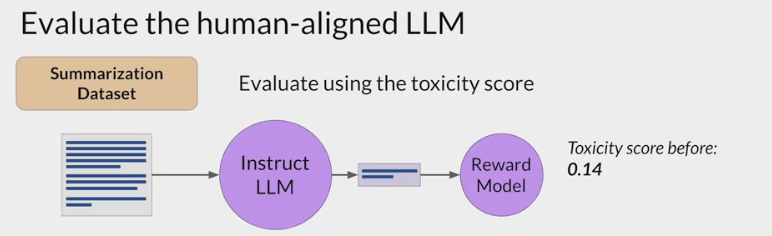
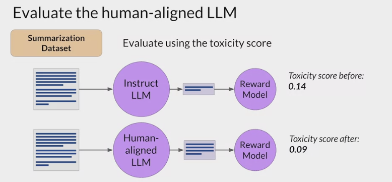
use the summarization data set to quantify the reduction in toxicity
- for example: use toxicity score, the probability of the negative class, a toxic or hateful response averaged across the completions.
- If RHF has successfully reduce the toxicity of the LLM, this score should go down.
- First, create a baseline toxicity score for the original instruct LLM by evaluating its completions off the summarization data set with a reward model that can assess toxic language.
- Then evaluate the newly human aligned model on the same data set and compare the scores.
- In this example, the toxicity score has indeed decreased after RLHF, indicating a less toxic, better aligned model.
Adapt and align large language models
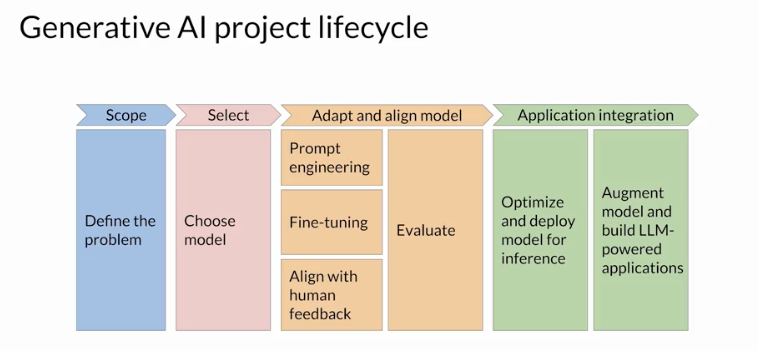
To integrate the model into applications.
- The first set is related to how the LLM will function in deployment.
- how fast do you need the model to generate completions?
- What compute budget do you have available?
- trade off model performance for improved inference speed or lower storage?
- The second set of questions is tied to additional resources that the model may need.
- Do you intend for the model to interact with external data or other applications?
- how will you connect to those resources?
- Lastly, how the model will be consumed.
- What will the intended application or API interface that the model will be consumed through look like?
Model optimization technique
Optimize the model before deploying it for inference.
- inference challenges:
- computing and storage
requirements
- ensuring low latency for consuming applications.
- computing and storage
- These challenges persist whether you’re deploying on premises or to the cloud
- become even more of an issue when deploying to edge devices.
- Optimizing the model for deployment will help ensure that the application functions well and provides the users with the best possible experience sense.
reduce the size of the LLM
One of the primary ways to improve application performance is to reduce the size of the LLM.
- allow for quicker loading of the model, reduces inference latency.
- the challenge:
reduce the size of the modelwhilemaintaining model performance. - three techniques
- all aim to reduce model size to improve model performance during inference without impacting accuracy.
- Distillation
- uses a larger model, the teacher model, to train a smaller model, the student model.
- use the smaller model for inference to lower the storage and compute budget.
- post training quantization
- transforms a model’s weights to a lower precision representation, such as a 16-bit floating point or eight bit integer.
- this reduces the memory footprint of the model.
- Model Pruning,
- removes redundant model parameters that contribute little to the model’s performance.
Model Distillation
- technique that focuses on having a larger teacher model train a smaller student model.
The student model learns to statistically mimic the behavior of the teacher model, either just in the final prediction layer or in the model’s hidden layers as well.
- in the final prediction layer
- start with the fine tune LLM (teacher model), create a smaller LLM (student model).
- freeze the teacher model’s weights, use it to generate completions for the training data.
- generate completions for the training data using the student model.
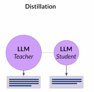
- The knowledge distillation between teacher and student model is achieved by minimizing a loss function: distillation loss .
- To calculate this loss, distillation uses the probability distribution over tokens that is produced by the teacher model’s softmax layer.
- the teacher model
- already fine tuned on the training data.
- So the probability distribution likely closely matches the ground truth data, won’t have much variation in tokens.
- That’s why Distillation applies a little trick adding a temperature parameter to the softmax function.
- a higher temperature increases the creativity of the language the model generates.
- With a temperature parameter greater than one, the probability distribution becomes broader and less strongly peaked.
- This softer distribution provides you with a set of tokens that are similar to the ground truth tokens.
- the teacher model’s output is often referred to as soft labels and the student model’s predictions as soft predictions.
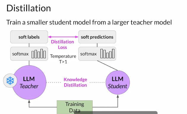
- In parallel, train the student model to generate the correct predictions based on the ground truth training data.
- don’t vary the temperature setting and instead use the standard softmax function.
- Distillation refers to the student model outputs as the hard predictions and hard labels .
- The loss between these two is the student loss.
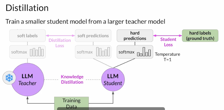
- The combined distillation and student losses are used to update the weights of the student model via back propagation.
- the smaller student model can be used for inference in deployment instead of the teacher model.
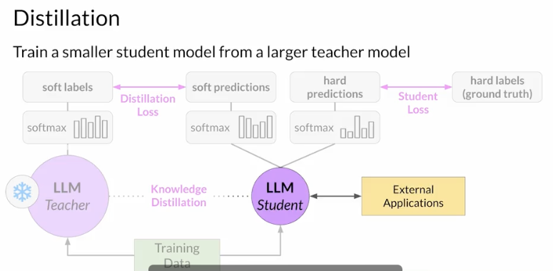
- In practice, distillation is not as effective for generative decoder models.
- It’s typically more effective for encoder only models,
- such as Burt that have a lot of representation redundancy.
- It’s typically more effective for encoder only models,
- with Distillation, you’re training a second, smaller model to use during inference.
- not reducing the model size of the initial LLM in any way.
PTQ - Post training quantization

- model optimization technique that actually reduces the size of the LLM .
- Specifically Quantization Aware Training / QAT
- after a model is trained, perform PTQ to optimize it for deployment.
- transforms a model’s weights to a lower precision representation, such as 16-bit floating point or 8-bit integer.
- To reduce the model size, memory footprint, and compute resources needed for model serving, quantization can be applied to just the model weights or to both weights and activation layers.
In general, quantization approaches that include the activations can have a higher impact on model performance.
- requires an extra calibration step to statistically capture the dynamic range of the original parameter values .
- sometimes quantization results in a small percentage reduction in model evaluation metrics.
- tradeoffs: if the reduction is worth the cost savings and performance gains .
Pruning
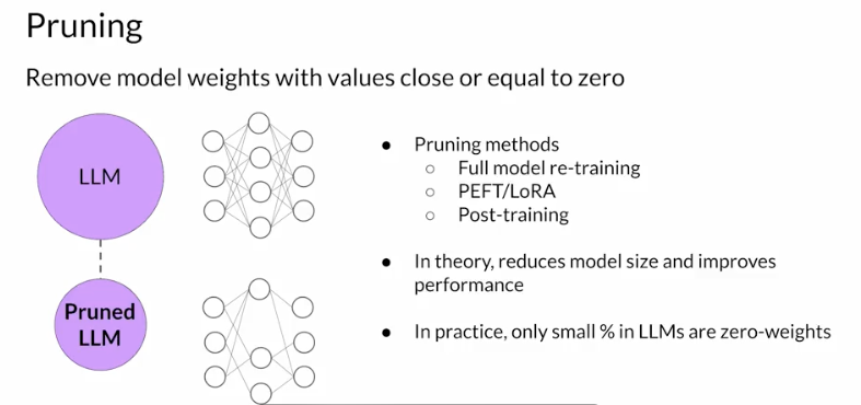
- reduce model size for inference by eliminating weights that are not contributing much to overall model performance .
- weights with values very close to or equal to zero.
- some pruning methods
- require
full retraining of the model - fall into the category of
parameter efficient fine tuning, such as LoRA. - methods that focus on post-training Pruning.
- require
- In theory, this reduces the size of the model and improves performance .
- In practice may not be much impact on the size and performance if only a small percentage of the model weights are close to zero .
Traning Terms
Epoch vs Batch Size vs Iterations 1
Gradient Descent
It is an iterative optimization algorithm used in machine learning to find the best results (minima of a curve).
Gradient: the rate of inclination or declination of a slope.Descent: the instance of descending.
The algorithm is iterative means that we need to get the results multiple times to get the most optimal result.
The iterative quality of the gradient descent helps a under-fitted graph to make the graph fit optimally to the data.
learning rate
- The Gradient descent has a parameter called
learning rate. - As you can see above (left), initially the steps are bigger that means the learning rate is higher and as the point goes down the learning rate becomes more smaller by the shorter size of steps.
- Also,the Cost Function is decreasing or the cost is decreasing
- Sometimes you might see people saying that the Loss Function is decreasing or the loss is decreasing, both Cost and Loss represent same thing (btw it is a good thing that our loss/cost is decreasing).
We need terminologies like epochs, batch size, iterations only when the data is too big which happens all the time in machine learning and we can’t pass all the data to the computer at once. So, to overcome this problem we need to divide the data into smaller sizes and give it to our computer one by one and update the weights of the neural networks at the end of every step to fit it to the data given.
Epochs
One Epoch is when an ENTIRE dataset is passed forward and backward through the neural network only ONCE.
Since one epoch is too big to feed to the computer at once we divide it in several smaller batches.
Why we use more than one Epoch?
- passing the entire dataset through a neural network is not enough.
- we need to pass the full dataset multiple times to the same neural network.
keep in mind that we are using a limited dataset and to optimise the learning and the graph we are using Gradient Descent which is an iterative process. So, updating the weights with single pass or one epoch is not enough.
One epoch leads to underfitting of the curve in the graph (below).
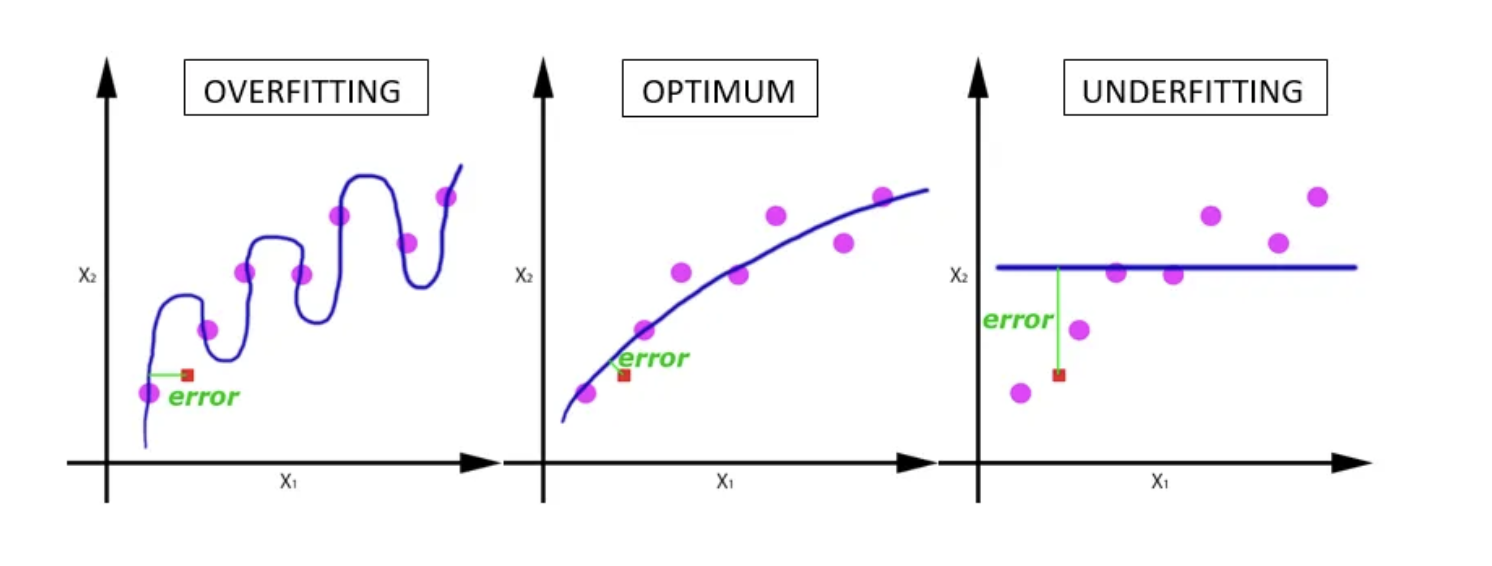
- As the number of epochs increases, more number of times the weight are changed in the neural network and the curve goes from underfitting to optimal to overfitting curve.
Right numbers of epochs?
- The answer is different for different datasets
- the numbers of epochs is related to how diverse the data is
- example:
- Do you have only black cats in the dataset or is it much more diverse dataset?
Batch Size
Total number of training examples present in a single batch.
Batch size and number of batches are two different things.
Batch:
you can’t pass the entire dataset into the neural net at once. So, you divide dataset into Number of Batches or sets or parts.
Just like you divide a big article into multiple sets/batches/parts like Introduction, Gradient descent, Epoch, Batch size and Iterations which makes it easy to read the entire article for the reader and understand it.
Iterations
Iterations is the number of batches needed to complete one epoch.
To get the iterations you just need to know multiplication tables or have a calculator.
the number of batches = the number of iterations for one epoch.
example:
- have 2000 training examples that we are going to use.
- divide the dataset of 2000 examples into batches of 500 then it will take 4 iterations to complete 1 epoch.
- Where Batch Size is 500 and Iterations is 4, for 1 complete epoch.
Q&A
- nB 大小的模型,训练和推理时,显存占用情况?
- 推理时显存的下限是 2nGB ,至少要把模型加载完全;训练时,如果用 Adam 优化器,参考前文的 2+2+12 的公式,训练时显存下限是 16nGB,需要把模型参数 梯度和优化器状态加载进来。
- 如果有 N 张显存足够大的显卡,怎么加速训练?
- 数据并行(DP),充分利用多张显卡的算力。
- 如果显卡的显存不够装下一个完整的模型呢?
- 最直观想法,需要分层加载,把不同的层加载到不同的 GPU 上(accelerate 的 device_map),也就是常见的 PP,流水线并行。
- 但 PP 推理起来,是一个串行的过程,1 个 GPU 计算,其他 GPU 空闲,有没有其他方式?
- 横向切分,流水线并行(PP),也就是分层加载到不同的显卡上;
- 纵向切分,张量并行(TP),也称作模型并行(MP)。
- 3 种并行方式可以叠加吗?
- 是可以的,DP+PP+TP,这就是 3D 并行。如果真有 1 个超大模型需要预训练,3D 并行那是必不可少的,参考 BLOOM 模型的训练,DP+PP 用 DeepSpeed,TP 用 Megatron-LM。
- 最主流的开源大模型?
- ChatGLM-6B,prefix LM;
- LLaMA-7B,causal LM。
- prefix LM 和 causal LM 的区别?
- Attention Mask 不同,前者的 prefix 部分的 token 互相能看到,后者严格遵守只有后面的 token 才能看到前面的 token 的规则。
- 哪种架构是主流?
- GPT 系列就是 Causal LM,目前除了 T5 和 GLM,其他大模型基本上都是 Causal LM。
- 如何给 LLM 注入领域知识?
- 第一种办法,检索+LLM,先用问题在领域数据库里检索到候选答案,再用 LLM 对答案进行加工;
- 第二种方法,把领域知识构建成问答数据集,用 SFT 让 LLM 学习这部分知识。
Epoch vs Batch Size vs Iterations, https://towardsdatascience.com/epoch-vs-iterations-vs-batch-size-4dfb9c7ce9c9 ↩
Comments powered by Disqus.