AI - AI
AIML - AI
Table of contents:
- AIML - AI
ref:
- OWAPS Top10 for LLM v1
- https://www.freecodecamp.org/news/large-language-models-and-cybersecurity/
- https://www.experts-exchange.com/articles/38220/Ensuring-the-Security-of-Large-Language-Models-Strategies-and-Best-Practices.html
- https://docs.whylabs.ai/docs/integrations-llm-whylogs-container
- https://hackernoon.com/security-threats-to-high-impact-open-source-large-language-models
- https://a16z.com/emerging-architectures-for-llm-applications/
- Examining Zero-Shot Vulnerability Repair with Large Language Models
- medusa
- awesome-generative-ai
- Google’s Secure AI Framework
- The Foundation Model Transparency Index
Link:
Overview
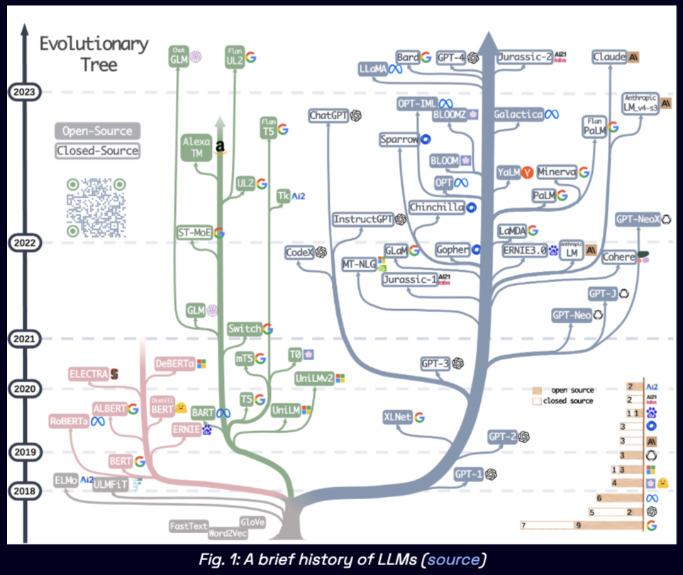
Research in artificial intelligence is increasing at an exponential rate. It’s difficult for AI experts to keep up with everything new being published, and even harder for beginners to know where to start.
- Transformers Neural Network
- After the big success of
Transformers Neural Network, it has been adapted to manyNatural Language Processing (NLP)tasks (such as question answering, text translation, automatic summarization)
“AI Canon”
- a curated list of resources we’ve relied on to get smarter about modern AI
- because these papers, blog posts, courses, and guides have had an outsized impact on the field over the past several years.
Data pipelines
- Databricks
- Airflow
- Unstructured
Embedding model
- OpenAI
- Cohere
- Hugging Face
Vector database
- Pinecone
- Weaviate
- ChromaDB
- pgvector
Playground
- OpenAI
- nat.dev
- Humanloop
Orchestration
- Langchain
- LlamaIndex
- ChatGPT
APIs/plugins
- Serp
- Wolfram
- Zapier
LLM cache
- Redis
- SQLite
- GPTCache
Logging / LLMops
- Weights & Biases
- MLflow
- PromptLayer
- Helicone
Validation
- Guardrails
- Rebuff
- Microsoft Guidance
- LMQL
App hosting
- Vercel
- Steamship
- Streamlit
- Modal
LLM APIs (proprietary)
- OpenAI
- Anthropic
LLM APIs (open)
- Hugging Face
- Replicate
Cloud providers
- AWS
- GCP
- Azure
- CoreWeave
Opinionated clouds
- Databricks
- Anyscale
- Mosaic
- Modal
- RunPod
OpenSource
- hugging face
- OpenAI
- Generative AI (answers for everything)
Programming
- python
- panda
AI modeling
- pyTorch
- Tensor flow (Google)
ML platforms
- Jupyter Notebooks
Time series
- Forecasting and predictive Analytics
Use case
- Supply Chain Management with GenAI
OpenSource -> fine tuning -> custom result
AI
- Artificial Intelligence refers to
the ability of computers to perform tasks that typically require human-level intellect. AI is useful in many contexts, from automation to problem solving and merely trying to understand how humans think.
But it is important to note that AI is only concerned with human intelligence for now – it could possibly go beyond that.
Many people correlate the word ‘Intelligence’ with only ‘Human Intelligence’. Just because a chicken may not be able to solve a mathematical equation doesn’t mean it won’t run when you chase it. It is ‘Intelligent’ enough to know it doesn’t want you to catch it 🐔🍗.
Intelligence spans a much wider spectrum, and practically expands to any living thing that can make decisions or carry out actions autonomously, even plants.
Divisions of AI
Artificial Intelligence is
centered around computers and their ability to mimic human actions and thought processes.Programming and experiments have allowed humans to produce ANI systems. These can do things like classifying items, sorting large amounts of data, looking for trends in charts and graphs, code debugging, and knowledge representation and expression. But computers don’t think like humans, they merely mimic humans.
This is evident in voice assistants such as
Google’s Assistant, Apple’s Siri, Amazon’s Alexa, and Microsoft’s Cortana. They are basic ANI programs that add ‘the human touch’. In fact, people are known to be polite to these systems simply because they combine computerized abilities with a human feel.These assistants have gotten better over the years but fail to reach high levels of sophistication when compared to their AGI counterparts.
There are two major divisions of AI:
Artificial Narrow Intelligence (ANI)
- focused on a small array of similar tasks or a small task that is programmed only for one thing.
- ANI is not great in dynamic and complex environments and is used in only areas specific to it.
- Examples include self-driving cars, as well as facial and speech recognition systems.
Artificial General Intelligence (AGI)
- focused on a wide array of tasks and human activities.
- AGI is currently theoretical and is proposed to adapt and carry out most tasks in many dynamic and complex environments.
- Examples include J.A.R.V.I.S from Marvel’s Iron Man and Ava from Ex-Machina.
Traditional AIML vs GenAI
Traditional AIML
- good at identify pattern
- learning from the pattern
- limit success with close supervised learning of very large amount of data
- must have human involved
GenAI
- produces ‘content’ (text, image, music, art, forecasts, etc…)
use ‘transformers’ (Encoders/Decoders) based on pre-trained data using small amount of fine tuning data
- encode and decode at the same time
- less data and faster
- GenAI use small data and uses encoders and decoders and Transformers to take that smaller data and be able to use it for other types of models. (Pre training)
- then add on top of it small amounts of fine tuning data
- and then get a a training model.
- As perceptions, not neurons.
- encode and decode at the same time
- Generative AI is a subset of traditional machine learning.
- And the generative AI machine learning models have learned these abilities by
finding statistical patterns in massive datasets of contentthat was originally generated by humans.
- And the generative AI machine learning models have learned these abilities by
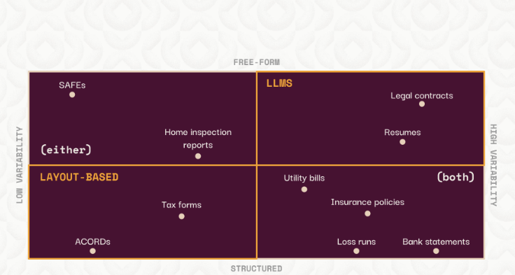
choosing between LLMs or layout-based Traditional AIML1
- recommends using LLM prompts for free-form, highly variable documents
- layout-based or “rule-based” queries for structured, less-variable documents.
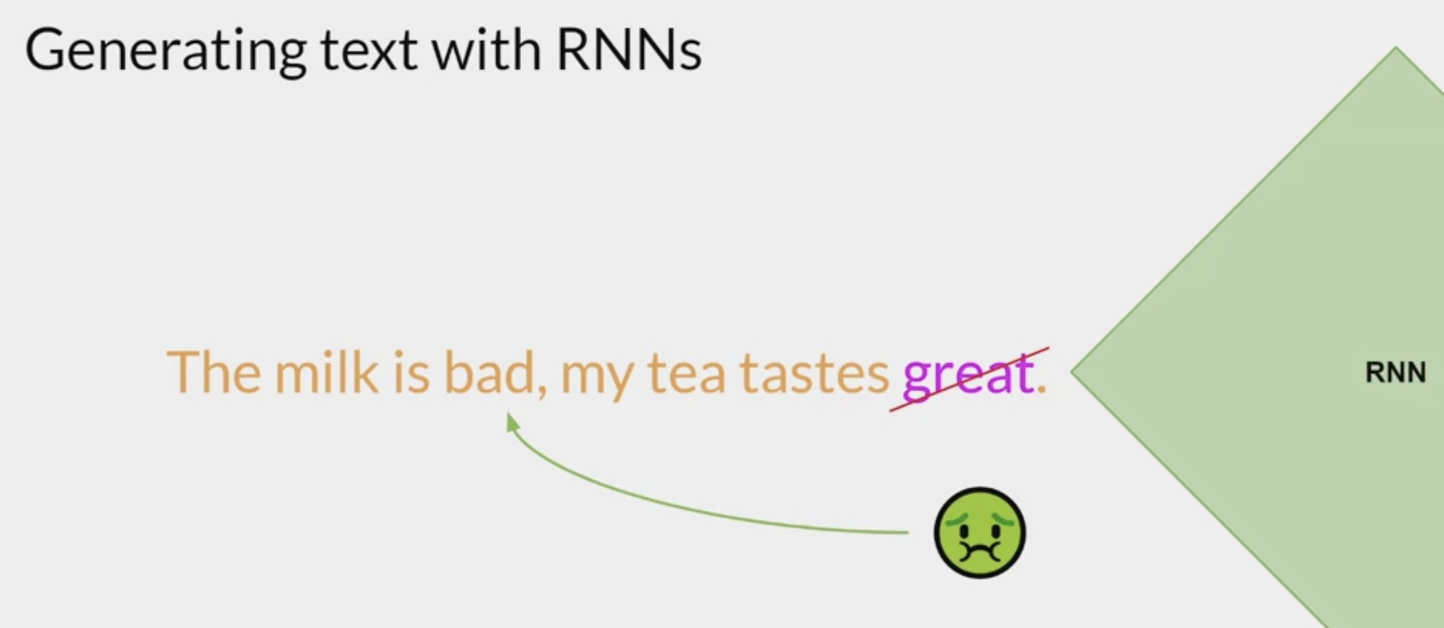
RNN - Recurrent neural networks
generative algorithms are not new.
recurrent neural networks - RNNs
- Previous generations of language models made use of an architecture called RNNs.
RNNs were limited by the amount of
compute and memoryneeded to perform well at generative tasks.- With just one previous words seen by the model, the prediction can’t be very good.
- scale the RNN implementation to be able to see more of the preceding words in the text,
- significantly scale the resources that the model uses.
- As for the prediction, Even though scale the model, it still hasn’t seen enough of the input to make a good prediction.
- To successfully predict the next word,
- models need to see more than just the previous few words.
- Models needs to have an understanding of the whole sentence or even the whole document.
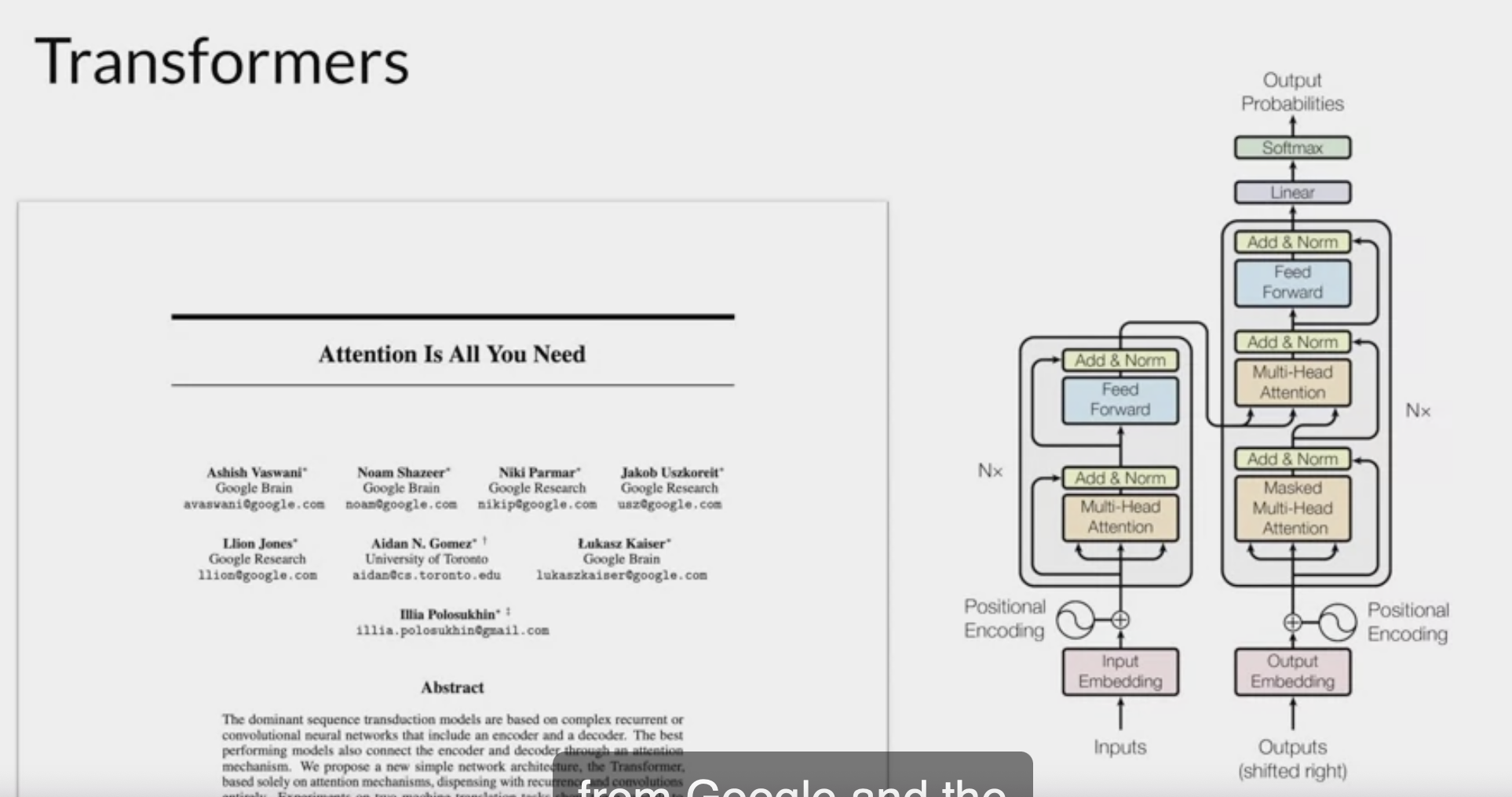
How can an algorithm make sense of human language if sometimes we can’t? in 2017, after the publication of this paper,
Attention is All You Need, from Google and the University of Toronto, everything changed. The transformer architecture had arrived.
- It can be scaled efficiently to use multi-core GPUs,
- parallel process input data, making use of much larger training datasets, and crucially,
- it’s able to learn to pay attention to the meaning of the words it’s processing.
Attention is all you need
High alignment
Multi-Headed Attention
名词解释
- LLM: Large Language Model,大型语言模型。
- PLM: Pretrain Language Model,预训练语言模型。
- RL: Reinforcement Learning,强化学习。
- SFT: Supervised Fine-Tuning,有监督微调。
ICL: In-Context Learning,上下文学习。
对比学习:
- 自监督学习(Self-supervised learning)可以避免对数据集进行大量的标签标注。
- 把自己定义的伪标签当作训练的信号,然后把学习到的表示(representation)用作下游任务里。
- 最近,对比学习被当作自监督学习中一个非常重要的一部分,被广泛运用在计算机视觉, 自然语言处理等领域。
- 它的目标是: 将一个样本的不同的, 增强过的新样本们在嵌入空间中尽可能地近,然后让不同的样本之间尽可能地远。
- SimCSE《SimCSE: Simple Contrastive Learning of Sentence Embeddings》是基于对比学习的表示学习方法,即采用对比学习的方法,获取更好的文本表征。
- SimCSE 细节可参考论文精读-SimCSE。
- Fine-Tuning : 微调。
- Prompt-Tuning: 提示微调。
Instruction-Tuning: 指示/指令微调。
- NLU: Natural Language Understanding,自然语言理解。
- NLG: Natural Language Generation,自然语言生成。
- CoT: Chain-of-Thought,思维链。
OOV:
- OOV 问题是 NLP 中常见的一个问题,其全称是 Out Of Vocabulary 超出词表外的词。
- 定义:
- 在自然语言处理过程中,通常会有一个字词库(vocabulary)。
- 这个 vocabulary 或者是提前加载的,或者是自己定义的,或者是从当前数据集提取的。
- 假设通过上述方法已经获取到一个 vocabulary,但在处理其他数据集时,发现这个数据集中有一些词并不在现有的 vocabulary 中,这时称这些词是 Out-Of-Vocabulary,即 OOV;
- 解决方法:
- Bert 中解决 OOV 问题。如果一个单词不在词表中,则按照 subword 的方式逐个拆分 token,如果连逐个 token 都找不到,则直接分配为[unknown]。
- shifted right: 指的是 Transformer Decoder 结构中,decoder 在之前时刻的一些输出,作为此时的输入,一个一个往右移。
- 重参数化: 常规思想: 对于网络层需要的参数是 $\Phi$,训练出来的参数就是 $\Phi$。重参数化方法: 训练时用的是另一套不同于 $\Phi$的参数,训练完后等价转换为 $\Phi$用于推理。
- PPL: 困惑度(Perplexity),用于评价语言模型的好坏。
- FCNN: Fully connected neural network,全连接神经网络。
- FNN: Feedforward neural network,前馈神经网络。
- DNN: Deep neural network,深度神经网络。
- MLP: Multi-layer perceptron neural networks,多层感知机。
- RM: Reward Model,奖励模型。
- PPO,Proximal Policy Optimization,近端策略优化,简单来说,就是对目标函数通过随机梯度下降进行优化。
- Emergent Ability: 很多能力小模型没有,只有当模型大到一定的量级之后才会出现。这样的能力称为涌现能力。
- AutoRegression Language Model: 自回归语言模型。
- Autoencoder Language Model: 自编码语言模型。
- CLM: Causal language modeling,因果语言建模,等价于 AutoRegression Language Model。
- AIGC: Artificial Intelligence Generated Content,生成式人工智能。
AGI: Artificial General Intelligence,通用人工智能。
- Bert;自编码模型,适用于 NLU(预训练任务主要挖掘句子之间的上下文关系) [^—步步走进Bert]
- GPT;自回归模型,适用于 NLG(预训练任务主要用于生成下文),有关 GPT 系列的理论知识,可参考本文的 GPT 系列章节;
GenAI
With the rise in popularity of Foundation Models, new models and tools are released almost every week and yet
- 就目前的发展趋势而言,大模型的训练基本就是按照Pretrain, Instruction-Tuning, RLHF三步走模式进行,因此技术上基本没什么问题,主要瓶颈存在于算力
对于中文大模型来说,获取高质量中文数据也是个问题。国内能耗费大规模成本进行大模型训练的厂商屈指可数
- 未来的发展趋势,可能有以下四个方向:
- 统一大模型: 头部企业逐步迭代出可用性很强的大语言模型(千亿级别),开放 API 或在公有云上供大家使用;
- 垂直领域模型: 部分企业逐步迭代出在相关垂直领域可用性很强的大语言模型(百亿级别),自用或私有化提供客户使用;
- 并行训练技术: 全新或更具可用性, 生态更完整的并行训练技术/框架开源,满足大部分有训练需求的企业/个人使用,逐步实现人人都能训练大模型;
- 颠覆: 或许某一天,横空出世的论文推翻了目前的大模型发展路线,转而证明了人们更需要的是另一种大模型技术,事情就会变得有意思了。
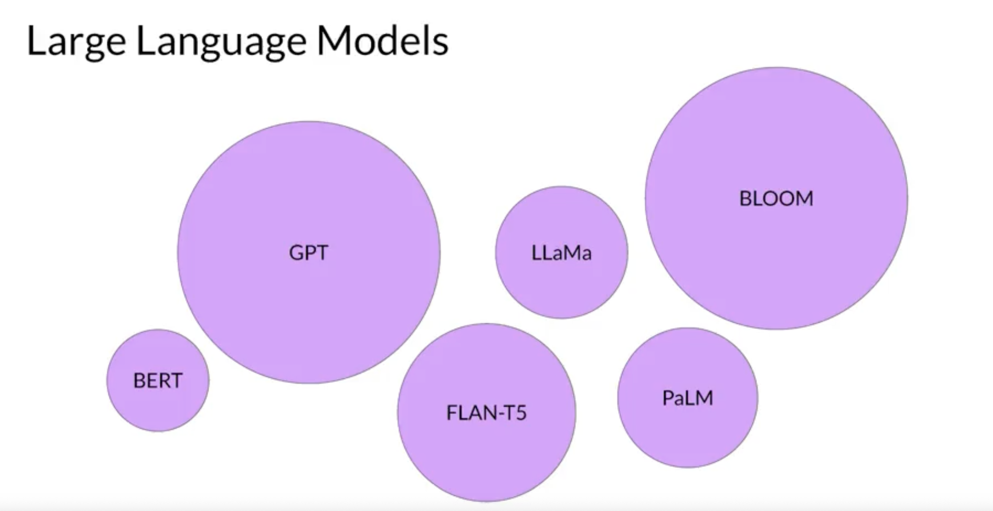
Large Language Model
“… a language model is a Turing-complete weird machine running programs written in natural language; when you do retrieval, you are not ‘plugging updated facts into the AI’, you are actually downloading random new unsigned blobs of code from the Internet (many written by adversaries) and casually executing them on the LM with full privileges. This does not end well.” - Gwern Branwen on LessWrong
a deep learning model which consists of a
neural networkwith billions of parameters, trained on distinctively large amounts of unlabelled data using self-supervised learning.At the core of all AI are algorithms. Algorithms are procedures or steps to carry out a specific task. The more complex the algorithm, the more tasks can be carried out and the more widely it can be applied. The aim of AI developers is to find the most complex algorithms that can solve and perform a wide array of tasks.
The procedure to create a basic fruit recognition model using an simple analogy:
- There are two people: A teacher and a bot creator
- The bot creator creates random bots, and the teacher teaches and tests them on identifying some fruits
- The bot with the highest test score is then sent back to the creator as a base to make new upgraded bots
- These new upgraded bots are sent back to the teacher for teaching and testing, and the one with the highest test score is sent back to the bot creator to make new better bots.
- This is an oversimplification of the process, but nevertheless it relays the concept. The Model/Algorithm/Bot is continuously trained, tested, and modified until it is found to be satisfactory. More data and higher complexity means more training time required and more possible modifications.
- the developer of the model can tweak a few things about the model but may not know how those tweaks might affect the results.
A common example of this are neural networks, which have hidden layers whose deepest layers and workings even the creator may not fully understand.
Self-supervised learning means that rather than the teacher and the bot creator being two separate people, it is one highly skilled person that can both create bots and teach them.
- This makes the process much faster and practically autonomous.
- The result is a bot or set of bots that are both sophisticated and complex enough to recognise fruit in dynamic and different environments.
In the case of LLMs, the data here are human text, and possibly in various languages. The reason why the data are large is because the LLMs take in huge amounts of text data with the aim of finding connections and patterns between words to derive context, meaning, probable replies, and actions to these text.
The results are models that seem to understand language and carry out tasks based on prompts they’re given.
Tuning 技术依赖于 LLM 的发展,同时也在推动着 LLM 的发展。
- 通常,LLM 指的是包含数百亿(或更多)参数的语言模型,这些模型在大量的文本数据上训练。
Features of LLMs
Information Retrieval
Translation
Text summarization
Invoke actions from text
- to invoke Apis, or some actions from elsewhere,
- connecting to resources that are based on the Internet.
Translation
- LLMs that are trained on an array of languages rather than just one can be used for translation from one language to another.
- It’s even theorised that large enough LLMs can find patterns and connections in other languages to derive meaning from unknown and lost languages, despite not knowing what each individual word may mean.
Automating Mundane Tasks 自动化日常任务
Task automation has always been a major aim of AI development. Language models have always been able to carry out syntax analysis, finding patterns in text and responding appropriately.
Large language models have an advantage with semantic analysis 语义分析, enabling the model to understand the underlying meaning and context, giving it a higher level of accuracy.
This can be applied to a number of basic tasks like
text summarising, text rephrasing, and text generation.
Emergent Abilities 新兴能力
Emergent Abilities are
unexpected but impressiveabilities LLMs have due to the high amount of data they are trained on.These behaviours are usually discovered when the model is used rather than when it is programmed.
Examples include multi-step arithmetic, taking college-level exams, and chain-of-thought prompting. 思维链提示
Drawbacks of LLMs
LLM Subject
Large language models
- Large language models have been trained on trillions of words over many weeks and months, and with large amounts of compute power.
- These foundation models with billions of parameters, exhibit emergent properties beyond language alone, and researchers are unlocking their ability to break down complex tasks, reason, and problem solve.
foundation models (base models)
- their relative size in terms of their parameters.
- parameters:
- the model’s
memory. - the more parameters a model has, the more memory, the more
sophisticatedthe tasks it can perform.
- the model’s
- By either using these models as they are or by applying fine tuning techniques to adapt them to the specific use case, you can rapidly
build customized solutions without the need to train a new modelfrom scratch.
Augmenting LLMs
- connecting LLM to external data sources or using them to invoke external APIs.
- use this ability to provide the model with information it doesn’t know from its pre-training and to enable the model to power interactions with the real-world.
Interact
other machine learning and programming paradigms: write computer code with formalized syntax to interact withlibraries and APIs.large language models: able to take natural language or human written instructions and perform tasks much as a human would.
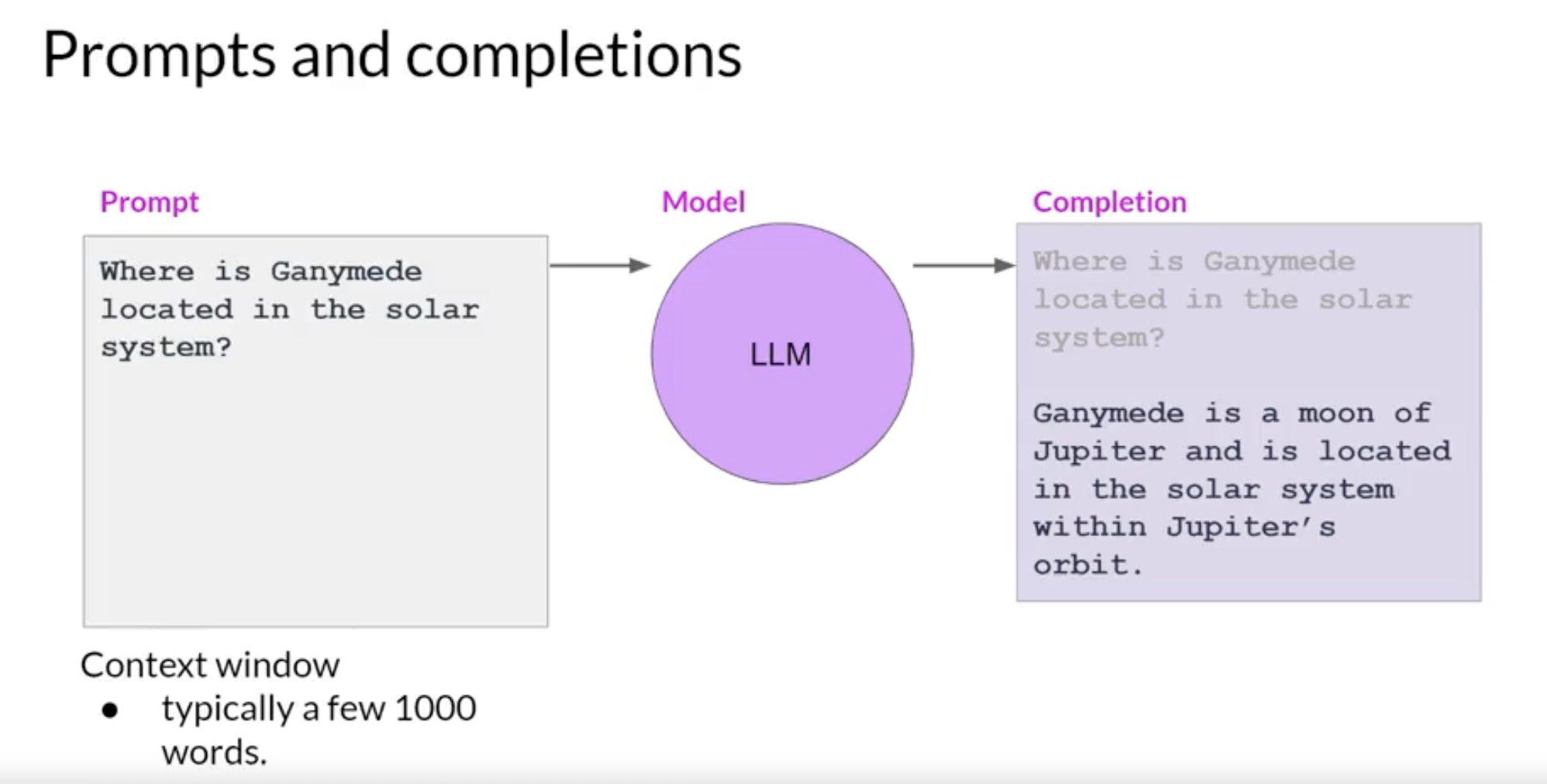
prompt
- The text that you pass to an LLM
The space or memory that is available to the prompt is called the
context window, and this is typically large enough for a few thousand words, but differs from model to model.- example
- ask the model to determine where Ganymede is located in the solar system.
- The prompt is passed to the model, the model then predicts the next words, and because the prompt contained a question, this model generates an answer.
- The output of the model is called a
completion, and the act of using the model to generate text is known asinference. - The completion is comprised of the text contained in the original prompt, followed by the generated text.
GPU
- cloud class instance (from NVIDIA)
- google colab
- kaggle
- amazon sagemaker
- gradient
- microsoft azure
Tesla is graphics cards from NVIDIA for AI
pyTorch
- it does these heavy mathematical computation very easily with libraries
- it got a whole set of APIs and utilities that let you manipulate all of these different tensors
tensors
- a tensor is a computer data object (data structure) that represents numeric data,
- it could be floating point data values or data objects within data objects.
- 1d tensors (column)
- 2d tensors (xy)
- 3d tensors (xyz)
- 4d tensors (cube)
- 5d tensors
- 6d tensors
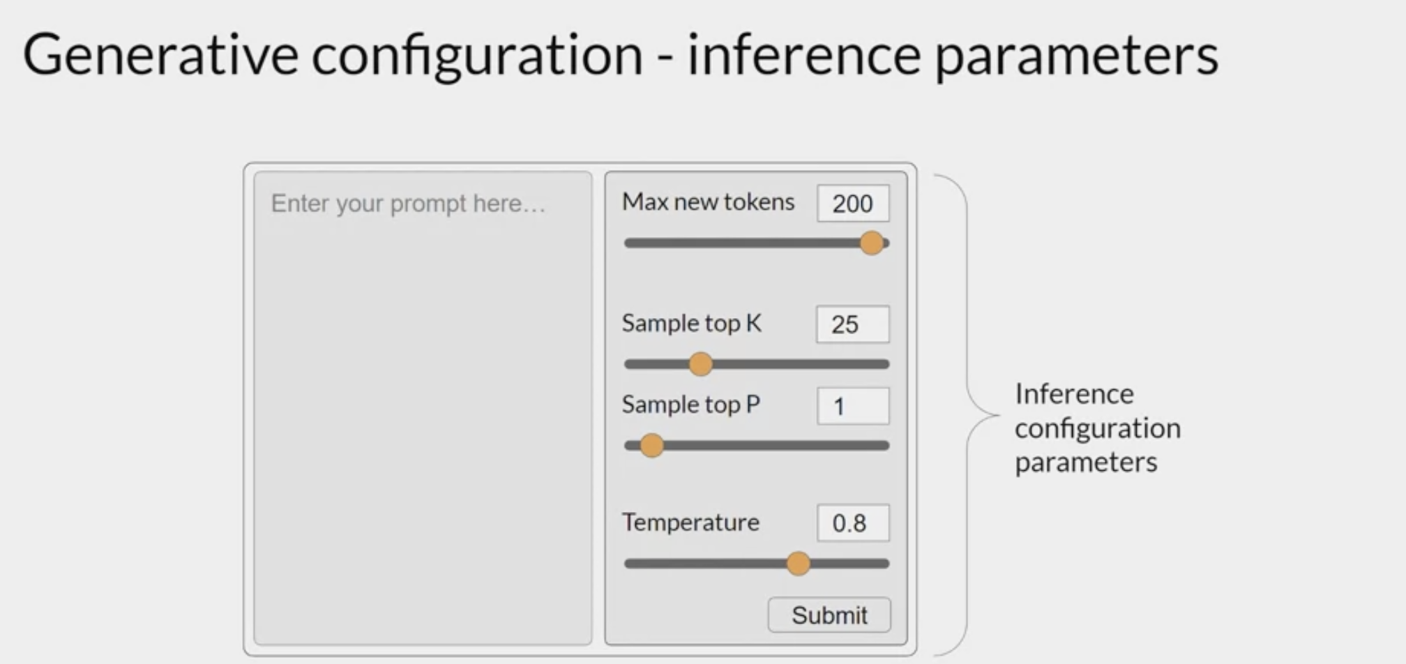
Generative configuration
- Each model exposes a set of configuration parameters that can influence the model’s output during inference.
- training parameters: learned during training time.
- configuration parameters: invoked at inference time and give control over things like the maximum number of tokens in the completion, and how creative the output is.
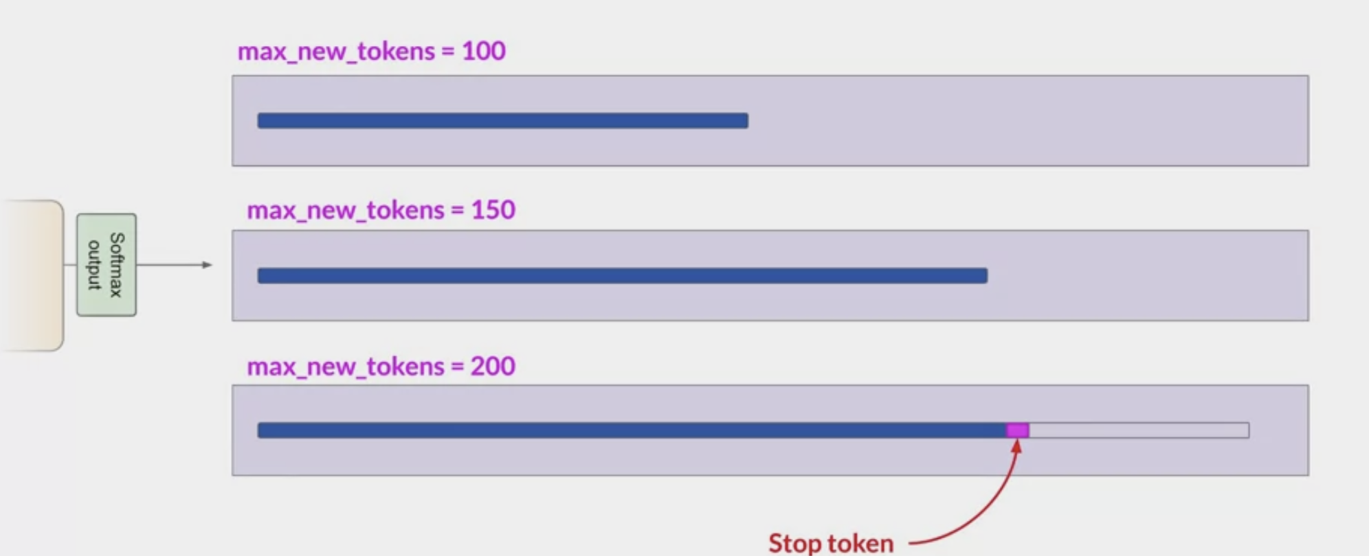
Max new tokens: limit the number of tokens that the model will generate.
- putting a cap on the number of times the model will go through the selection process.
the length of the completion is shorter
- because another stop condition was reached, such as the model predicting and end of sequence token.
- it’s max new tokens, not a hard number of new tokens generated.
- The output from the
transformer's softmax layeris aprobability distributionacross the entire dictionary of words that the model uses.- Here you can see a selection of words and their probability score next to them.
- this is a list that carries on to the complete dictionary.
controls
to generate text that’s more natural, more creative and avoids repeating words, you need to use some other controls.
- in some implementations, you may need to disable greedy and enable random sampling explicitly.
- For example, the Hugging Face transformers implementation that we use in the lab requires that we set do sample to equal true.
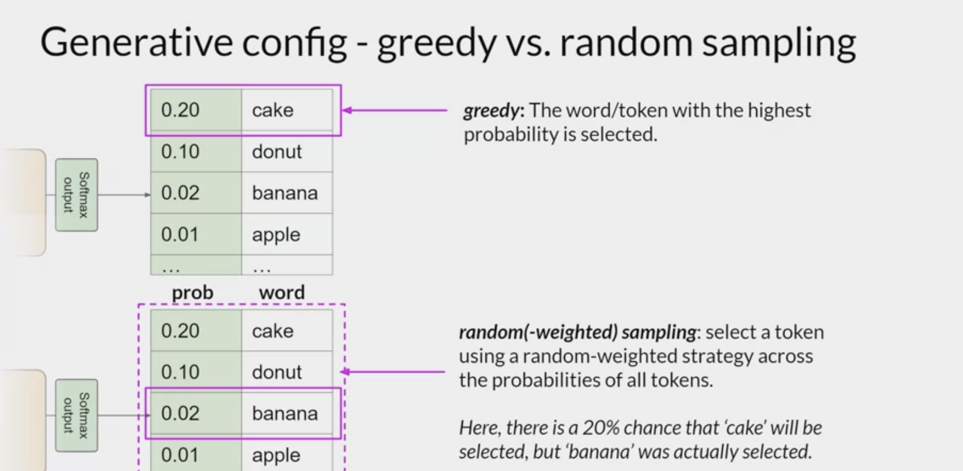
greedy decoding- Most large language models by default will operate with
greedy decoding. - the simplest form of next-word prediction
- the model will always choose the word with the highest probability.
- This method can work very well for short generation but is susceptible to repeated words or repeated sequences of words.
- Most large language models by default will operate with
Random sampling- the easiest way to introduce some variability.
- Instead of selecting the most probable word every time with random sampling, the model
chooses an output word at random using the probability distribution to weight the selection. depending on the setting, there is a possibility that the output may be too creative, producing words that cause the generation to wander off into topics or words that just don’t make sense.
For example, in the illustration, the word banana has a probability score of 0.02. With random sampling, this equates to a 2% chance that this word will be selected. By using this sampling technique, we reduce the likelihood that words will be repeated.
top k, top p sampling techniques
help
limit the random samplingandincrease the chance that the output will be sensible.- With
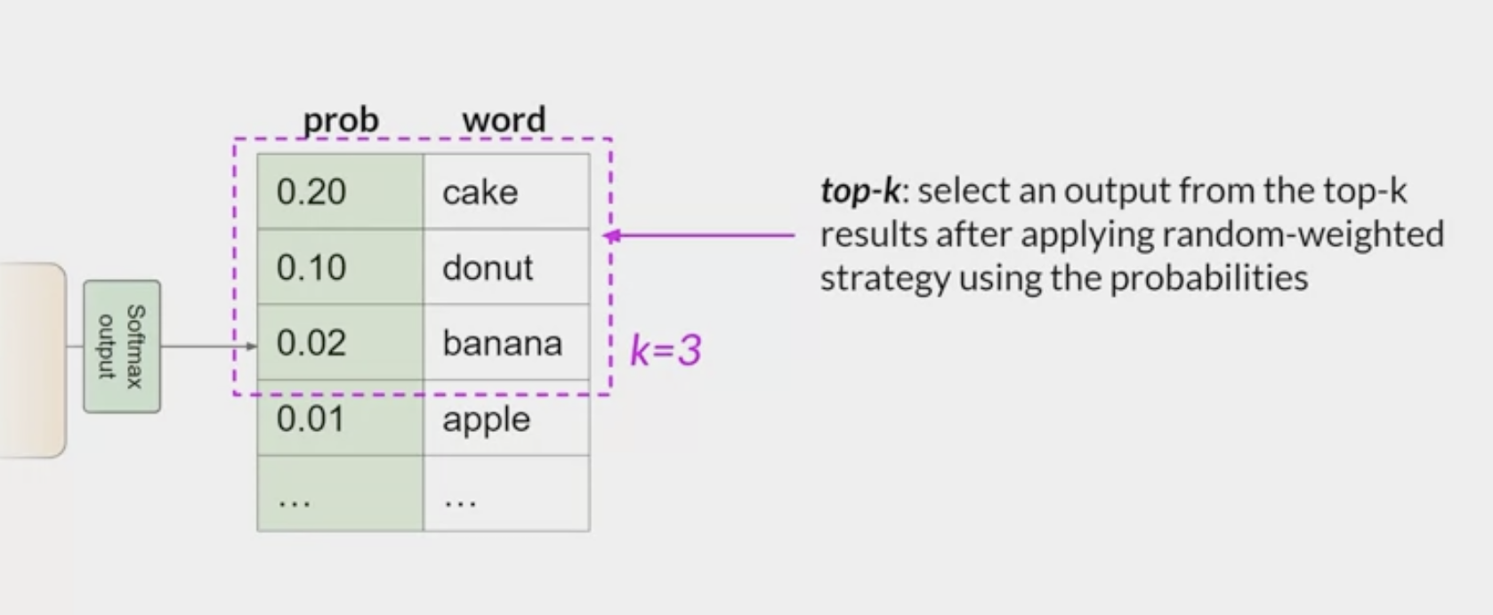
top k, you specify the number of tokens to randomly choose from - with
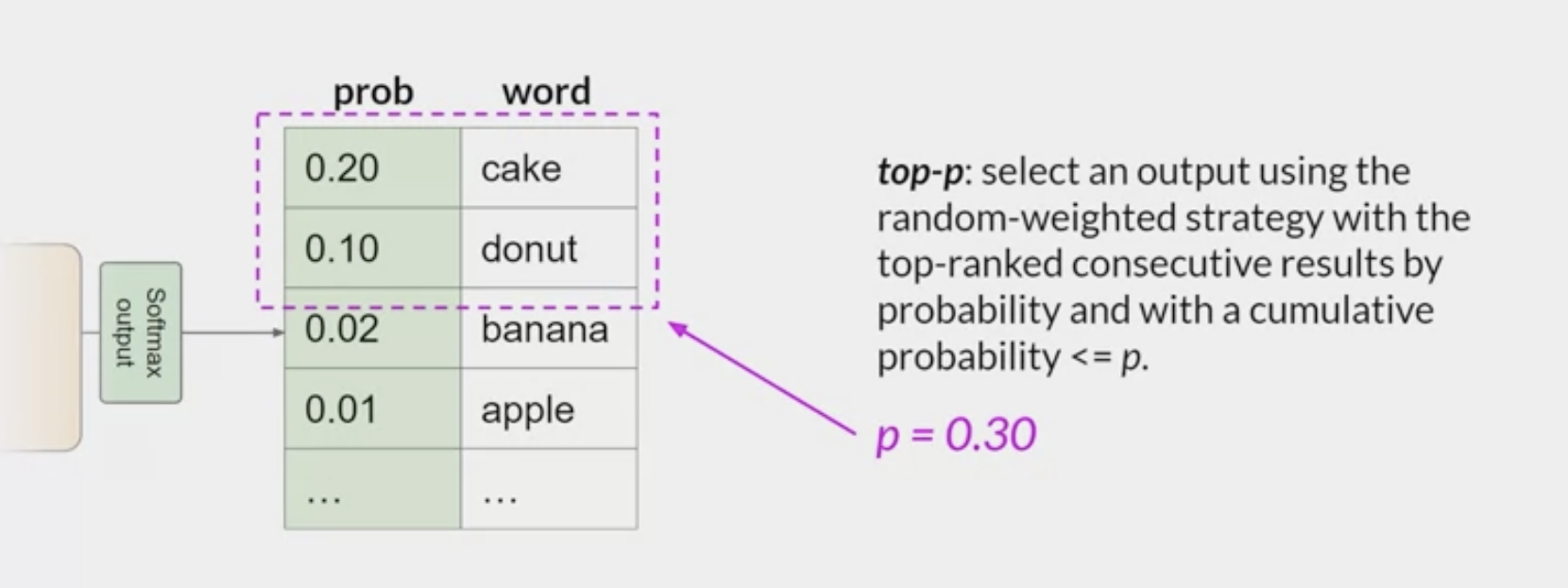
top p, you specify the total probability that you want the model to choose from.
- With
top kvalue:- limit the options while still allowing some variability
- instructs the model to choose from only the k tokens with the highest probability.
- In this example here, k is set to three, so you’re restricting the model to choose from these three options. The model then selects from these options using the probability weighting and in this case, it chooses donut as the next word.
- This method can help the model have some randomness while preventing the selection of highly improbable completion words.
- This in turn makes the text generation more likely to sound reasonable and to make sense.
top psetting:- limit the random sampling to the predictions whose combined probabilities do not exceed p.
- For example, if you set p to equal 0.3, the options are cake and donut since their probabilities of 0.2 and 0.1 add up to 0.3. The model then uses the random probability weighting method to choose from these tokens.
temperature
- control the randomness of the model output
can be adjusted to either increase or decrease randomness within the model output layer (softmax layer)
influences
the shape of the probability distributionthat the model calculates for the next token.- The temperature value is a
scaling factor that's applied within the final softmax layer of the modelthat impactsthe shape of the probability distribution of the next token. - In contrast to the
top k & pparameters, changing the temperature actually alters the predictions that the model will make.
- The temperature value is a
- Broadly speaking, the higher the temperature, the higher the randomness, and the lower the temperature, the lower the randomness.
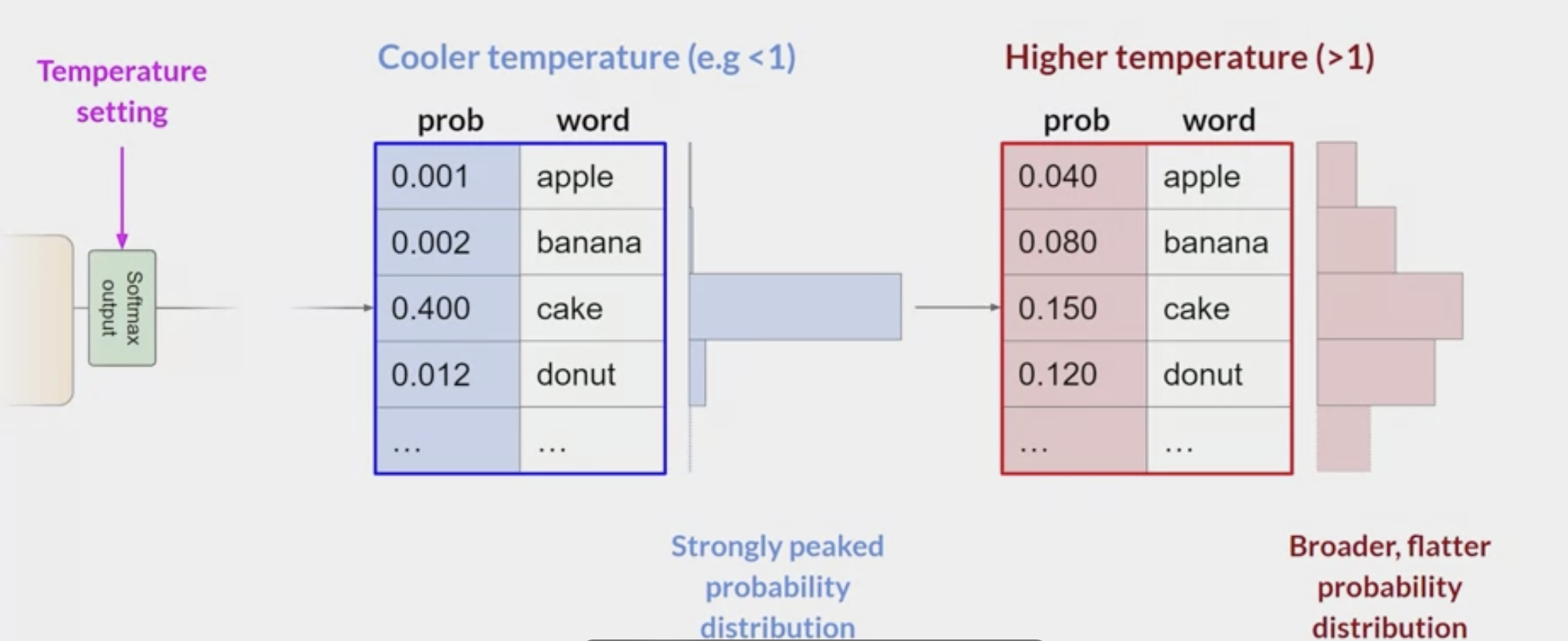
low value of temperature, say less than one,
- the resulting probability distribution from the softmax layer is more strongly peaked with the probability being concentrated in a smaller number of words.
- blue bars in the table show a probability bar chart turned on its side.
- Most of the probability here is concentrated on the word cake. The model will select from this distribution using random sampling and the resulting text will be less random and will more closely follow the most likely word sequences that the model learned during training.
if set the temperature to a higher value, say, greater than one, then the model will calculate a broader flatter probability distribution for the next token.
- Notice that in contrast to the blue bars, the probability is more evenly spread across the tokens.
- This leads the model to generate text with a
higher degree of randomness and more variabilityin the output compared to acool temperature setting. - This can help you generate text that sounds more creative.
- If leave the temperature value equal to one, this will leave the softmax function as default and the unaltered probability distribution will be used.
1
2
3
4
5
6
7
8
9
10
11
12
13
14
15
16
17
18
19
generation_config = GenerationConfig(max_new_tokens=50)
# generation_config = GenerationConfig(max_new_tokens=10)
# generation_config = GenerationConfig(max_new_tokens=50, do_sample=True, temperature=0.1)
# generation_config = GenerationConfig(max_new_tokens=50, do_sample=True, temperature=0.5)
# generation_config = GenerationConfig(max_new_tokens=50, do_sample=True, temperature=1.0)

inputs = tokenizer(few_shot_prompt, return_tensors='pt')
output = tokenizer.decode(
    model.generate(
        inputs["input_ids"],
        generation_config=generation_config,
    )[0],
    skip_special_tokens=True
)

print(dash_line)
print(f'MODEL GENERATION - FEW SHOT:\n{output}')
print(dash_line)
print(f'BASELINE HUMAN SUMMARY:\n{summary}\n')
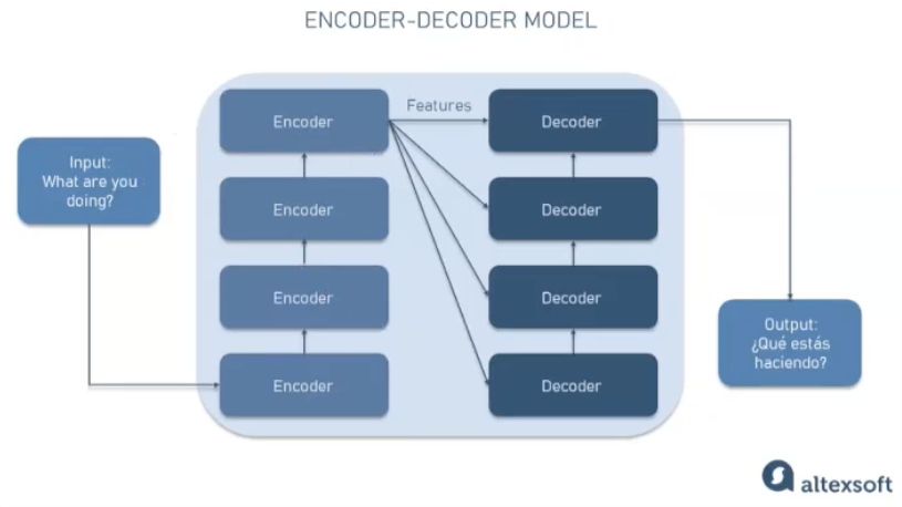
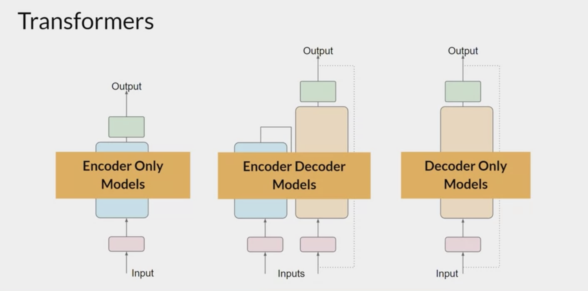
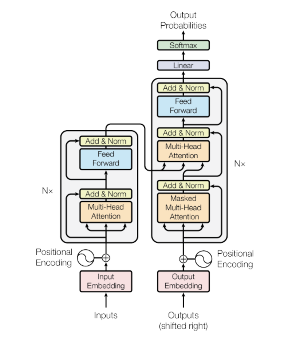
Encoder & Decoder
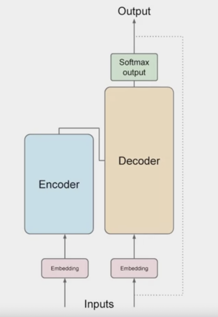
The transformer architecture is split into two distinct parts
- the encoder and the decoder.
- These components work in conjunction with each other and they share a number of similarities.
The encoder
encodes input sequences into a deep representation of the structure and meaning of the input.The decoder, working from input token triggers,
uses the encoder's contextual understanding to generate new tokens.It does this in a loop until some stop condition has been reached.
the inputs to the model are at the bottom and the outputs are at the top
Encoder vs Decoder
- Autoencoder models
- referred to as a Masked Language Model (MLM),
- the model is trained to predict masked tokens (tokens that have been intentionally masked out) in a sequence.
- This approach helps the model learn bidirectional relationships between tokens in the input sequence.
- Autoregressive models
- use causal language modeling with the objective to guess the next token based on the previous sequence of tokens.
- focus on predicting the next token or word making them best suited for text generation tasks.
- sequence-to-sequence (Seq2Seq) models
- These models can take an input sequence (e.g., a sentence in one language) and generate an output sequence (e.g., the translated sentence in another language) in a parallel and efficient manner .
- They achieve this by employing an encoder-decoder architecture with attention mechanisms, which allows them to handle variable-length input and output sequences effectively.
- well-suited to the task of text translation
Encoder-only models
- also work as sequence-to-sequence (Seq2Seq) models
- particularly those based on transformers, are widely used for tasks such as text translation.
- without further modification, the input sequence and the output sequence or the same length, less common these days,
- by adding additional layers to the architecture, you can train encoder-only models to perform
classification taskssuch as sentiment analysis, - encoder-only model example: BERT
Encoder-decoder models
- perform well on sequence-to-sequence tasks such as
translation - the input sequence and the output sequence can be different lengths.
- You can also scale and train this type of model to perform
general text generation tasks. - encoder-decoder models examples: BART, T5
- perform well on sequence-to-sequence tasks such as
- decoder-only models
- the most commonly used today.
- as they have scaled, their capabilities have grown. These models can now generalize to most tasks.
- Popular decoder-only models: GPT family of models, BLOOM, Jurassic, LLaMA, and many more.
LLM 为什么都用 Decoder only 架构?[^LLM为什么都用Decoderonly架构]
- 训练效率和工程实现上的优势
- 在理论上是因为 Encoder 的双向注意力会存在低秩问题,这可能会削弱模型表达能力;
- 另一方面,就生成任务而言,引入双向注意力并无实质好处。
- 而 Encoder-Decoder 架构之所以能够在某些场景下表现更好,大概只是因为它多了一倍参数。
- 所以,在同等参数量, 同等推理成本下,Decoder-only 架构就是最优选择了。
- 训练效率: Decoder-only 架构只需要进行单向的自回归预测,而 Encoder-Decoder 架构需要进行双向的自编码预测和单向的自回归预测,计算量更大;
- 工程实现: Decoder-only 架构只需要一个模块,而 Encoder-Decoder 架构需要两个模块,并且需要处理两者之间的信息传递和对齐,实现起来更复杂;
- 理论分析: Encoder 的双向注意力会存在低秩问题,即注意力矩阵的秩随着网络深度的增加而降低2,结论是如果没有残差连接和 MLP 兜着,注意力矩阵会朝秩为 1 的矩阵收敛,最后每个 token 的表示都一样了,网络就废了,这可能会削弱模型的表达能力。而 Decoder 的单向注意力则不存在这个问题;
- 生成任务: 对于文本生成任务,Encoder 的双向注意力并无实质好处,因为它会引入右侧的信息,破坏了自回归的假设。而 Decoder 的单向注意力则可以保持自回归的一致性。
How the model works
machine-learning models are just big statistical calculators and they work with numbers, not words.
Tokenize:
- Before passing texts into the model to process, must first tokenize the words.
- converts the words into numbers
each number representing a position in a dictionary of all the possible words that the model can work with.
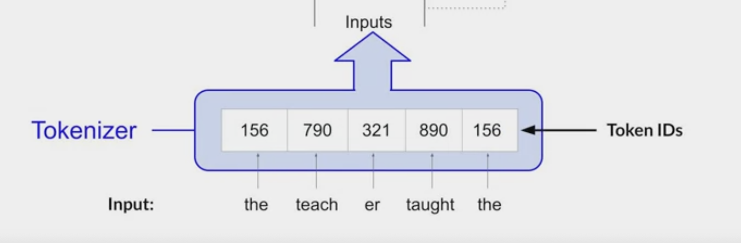
You can choose from multiple tokenization methods. For example,
- token IDs matching two complete words,
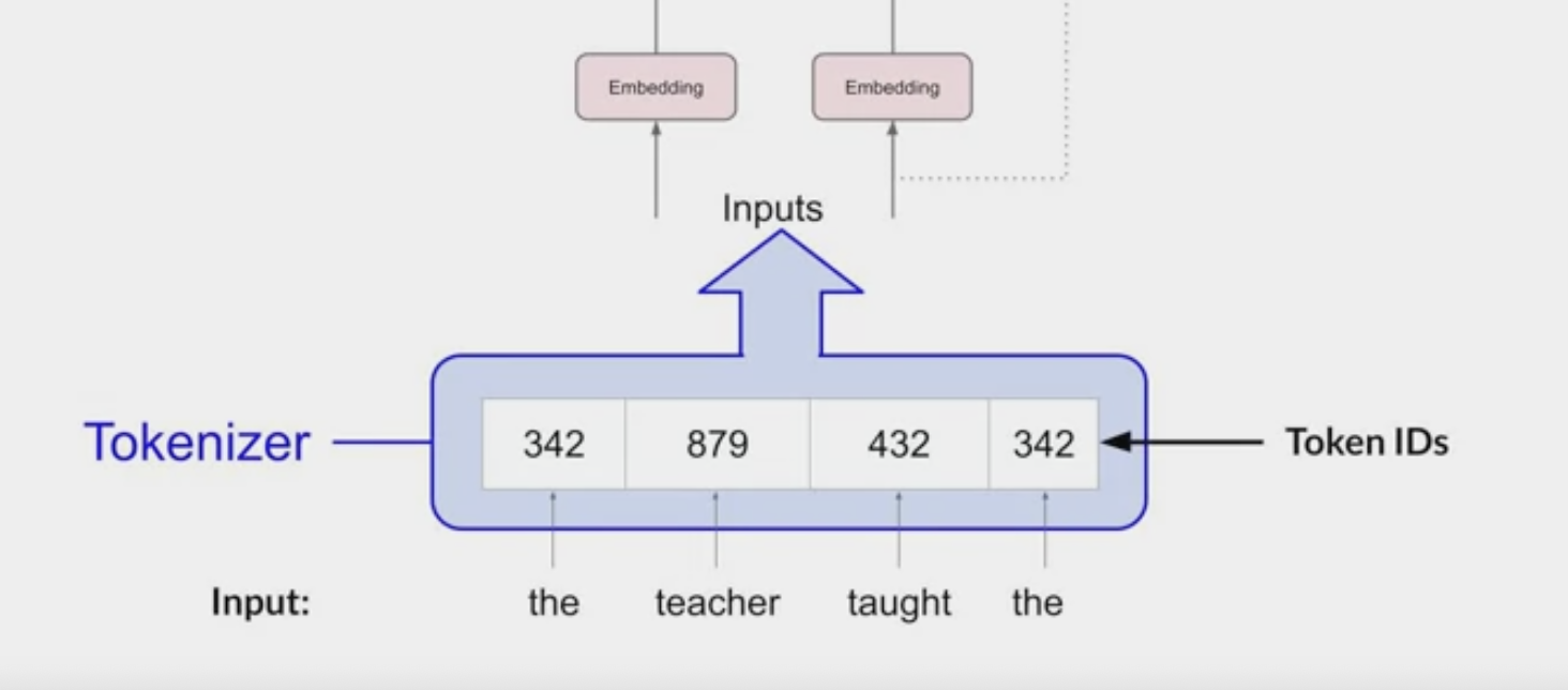
- or using token IDs to represent parts of words.
- once you’ve selected a tokenizer to train the model, you must use the same tokenizer when you generate text.
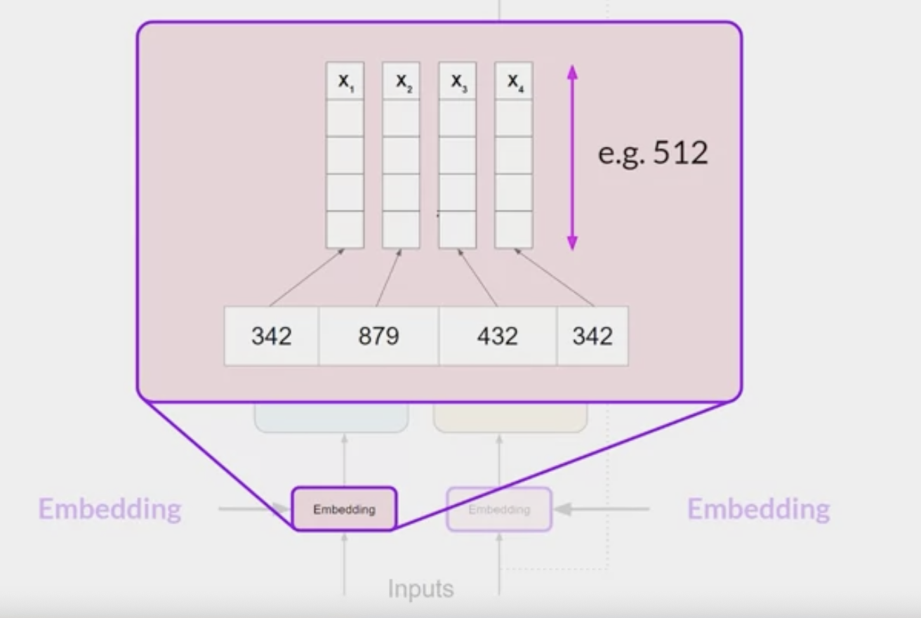
Token Embedding:
- Now that the input is represented as numbers, pass it to the embedding layer.
- This layer is a
trainable vector embedding space, - high-dimensional space where each token is represented as a vector and occupies a unique location within that space.
Each token ID in the vocabulary is matched to a
multi-dimensional vector, and the intuition is that these vectors learn toencode the meaning and context of individual tokens in the input sequence.Embedding vector spaces have been used in natural language processing for some time, previous generation language algorithms like Word2vec use this concept.
each word has been matched to a token ID, and each token is mapped into a vector.
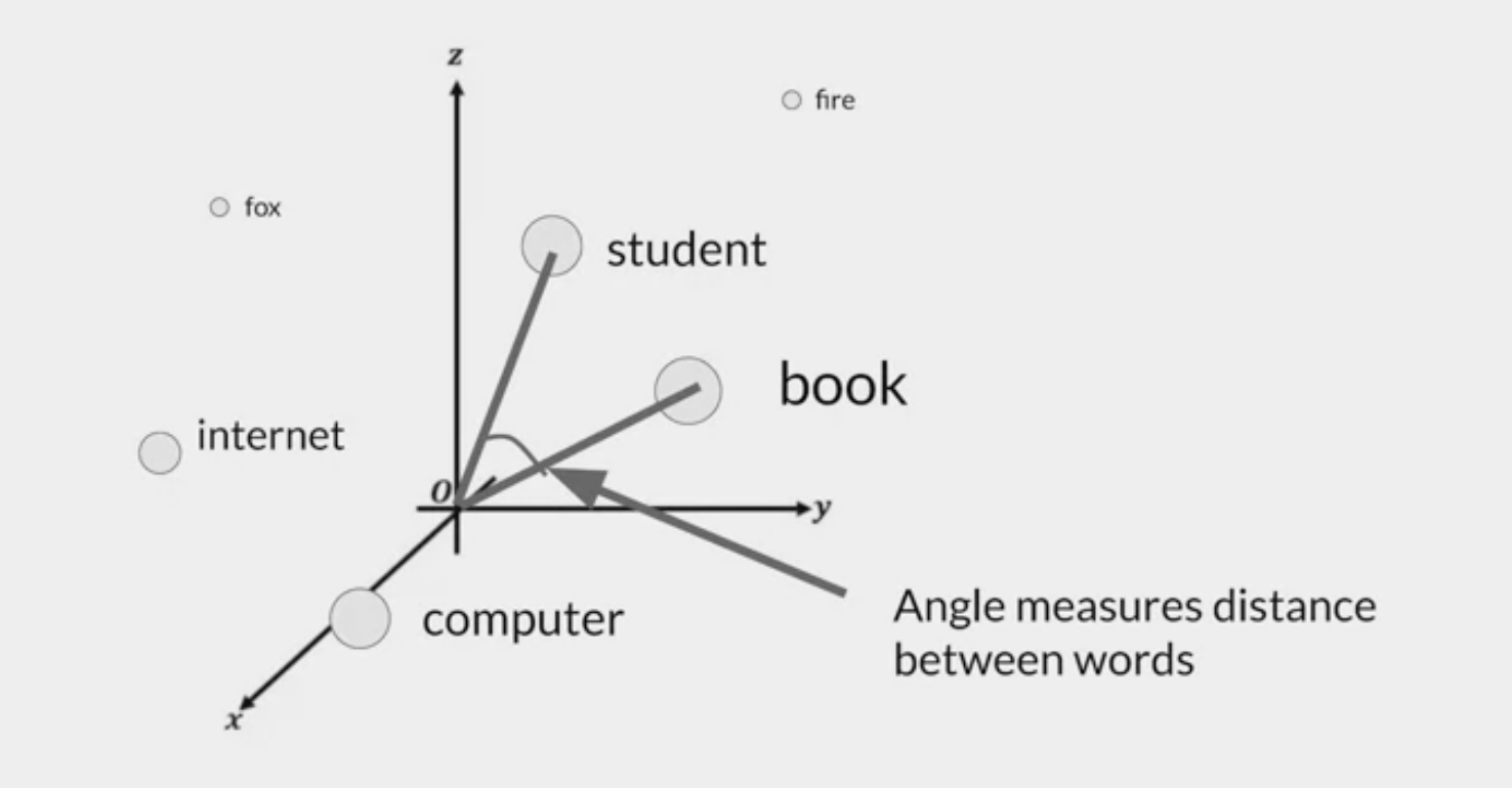
- In the original transformer paper, the vector size was actually 512
- For simplicity
- imagine a vector size of just three, you could plot the words into a three-dimensional space and see the relationships between those words.
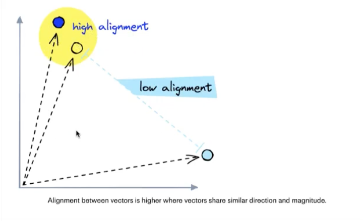
- relate words that are located close to each other in the embedding space, and calculate the distance between the words as an angle, which gives the model the ability to mathematically understand language.
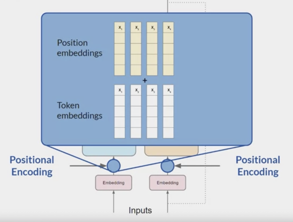
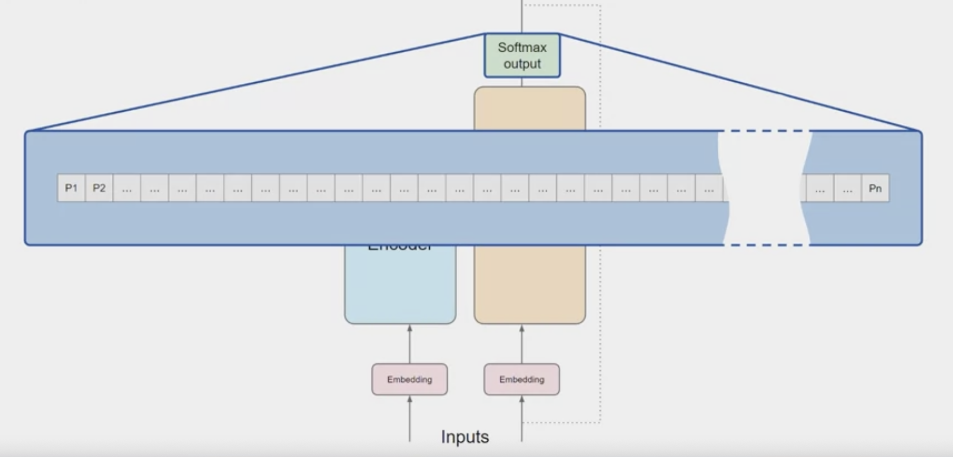
Positional Encoding:
- Added the token vectors into
the base of the encoder or the decoder, also add positional encoding. - The model processes each of the input tokens in parallel.
- it preserve the information about the word order and don’t lose the relevance of the position of the word in the sentence.
- Added the token vectors into
Self-attention
A mechanism that allows a model to focus on
different partsof the input sequence during computation.enables the transformer to weigh the importance of different tokens in the input sequence when processing each token
- allow the model to capture dependencies and relationships between tokens regardless of their distance in the sequence
sum the
input tokensand thepositional encodings, pass the resulting vectors to the self-attention layer.the model analyzes the relationships between the tokens in the input sequence, it allows the model to attend to different parts of the input sequence to better capture the contextual dependencies between the words.
The
self-attention weightsthat are learned during training and stored in these layers reflectthe importance of each word in that input sequence to all other words in the sequence.
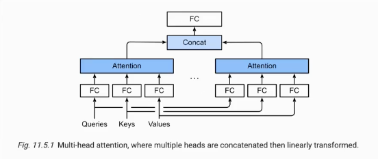
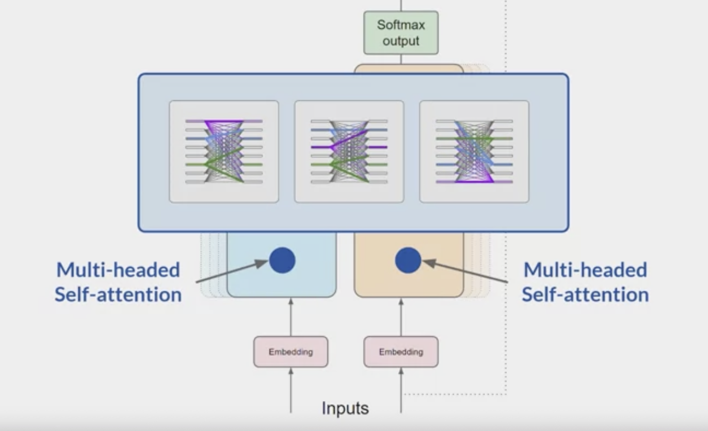
- But this does not happen just once, the transformer architecture actually has
multi-headed self-attention. 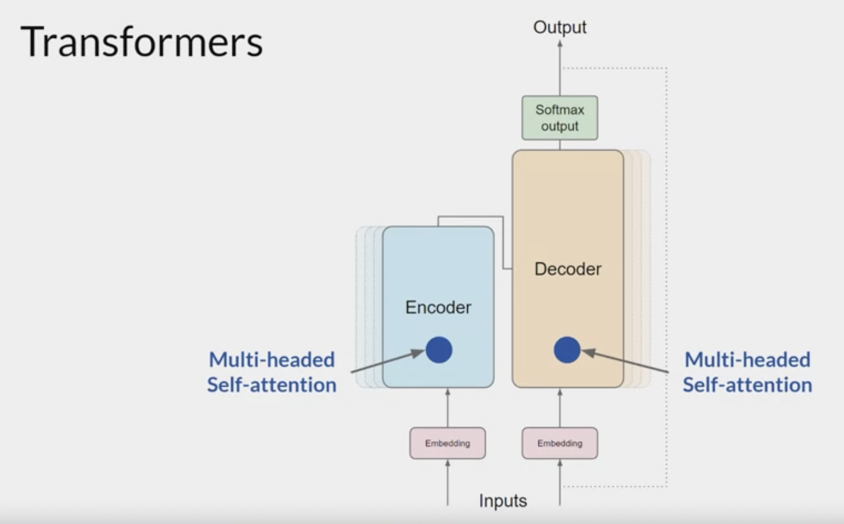
This means that
multiple sets of self-attention weights or headsare learned in parallel independently of each other.The number of attention heads included in the attention layer varies from model to model, but numbers in the range of 12-100 are common.
each self-attention head will learn a different aspect of language. For example,
- one head may see the relationship between the people entities in our sentence.
- another head may focus on the activity of the sentence.
- another head may focus on some other properties such as if the words rhyme.
don’t dictate ahead of time what aspects of language the attention heads will learn.
- The weights of each head are randomly initialized and given sufficient training data and time,
- each will learn different aspects of language.
- While some attention maps are easy to interpret, like the examples discussed here, others may not be.
- Now that all of the attention weights have been applied to the input data, the output is processed through a
fully-connected feed-forward network. 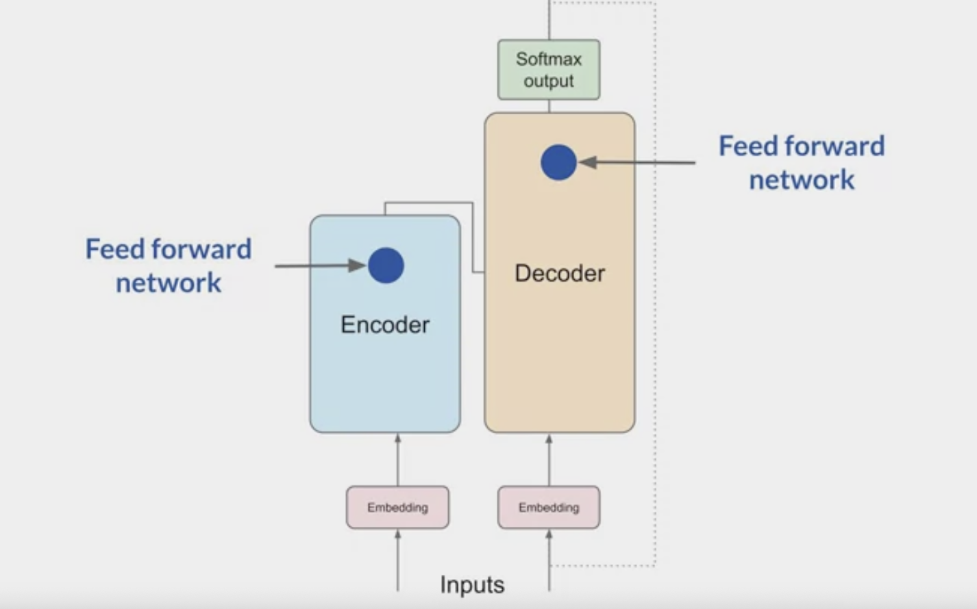
- The output of this layer is a vector of logits proportional to the probability score for each and every token in the tokenizer dictionary
Softmax
- then pass these logits to a final softmax layer, where they are normalized into a
probability score for each word. - This output includes a probability for every single word in the vocabulary, so there’s likely to be thousands of scores here.
- One single token will have a score higher than the rest.
- This is the most likely predicted token.
there are a number of methods that you can use to vary the final selection from this vector of probabilities.
- then pass these logits to a final softmax layer, where they are normalized into a
Overview prediction process
At a very high level, the workflow can be divided into three stages:
Data preprocessing / embedding:
- This stage involves storing private data to be retrieved later.
- Typically, the documents are broken into chunks, passed through an embedding model, then stored in a specialized database called a vector database.
Prompt construction / retrieval:
- When a user submits a query, the application constructs a series of prompts to submit to the language model.
- A compiled prompt typically combines
- a prompt template hard-coded by the developer;
- examples of valid outputs called few-shot examples;
- any necessary information retrieved from external APIs;
- and a set of relevant documents retrieved from the vector database.
Prompt execution / inference:
- Once the prompts have been compiled, they are submitted to a pre-trained LLM for inference—including both proprietary model APIs and open-source or self-trained models.
- Some developers also add operational systems like logging, caching, and validation at this stage.
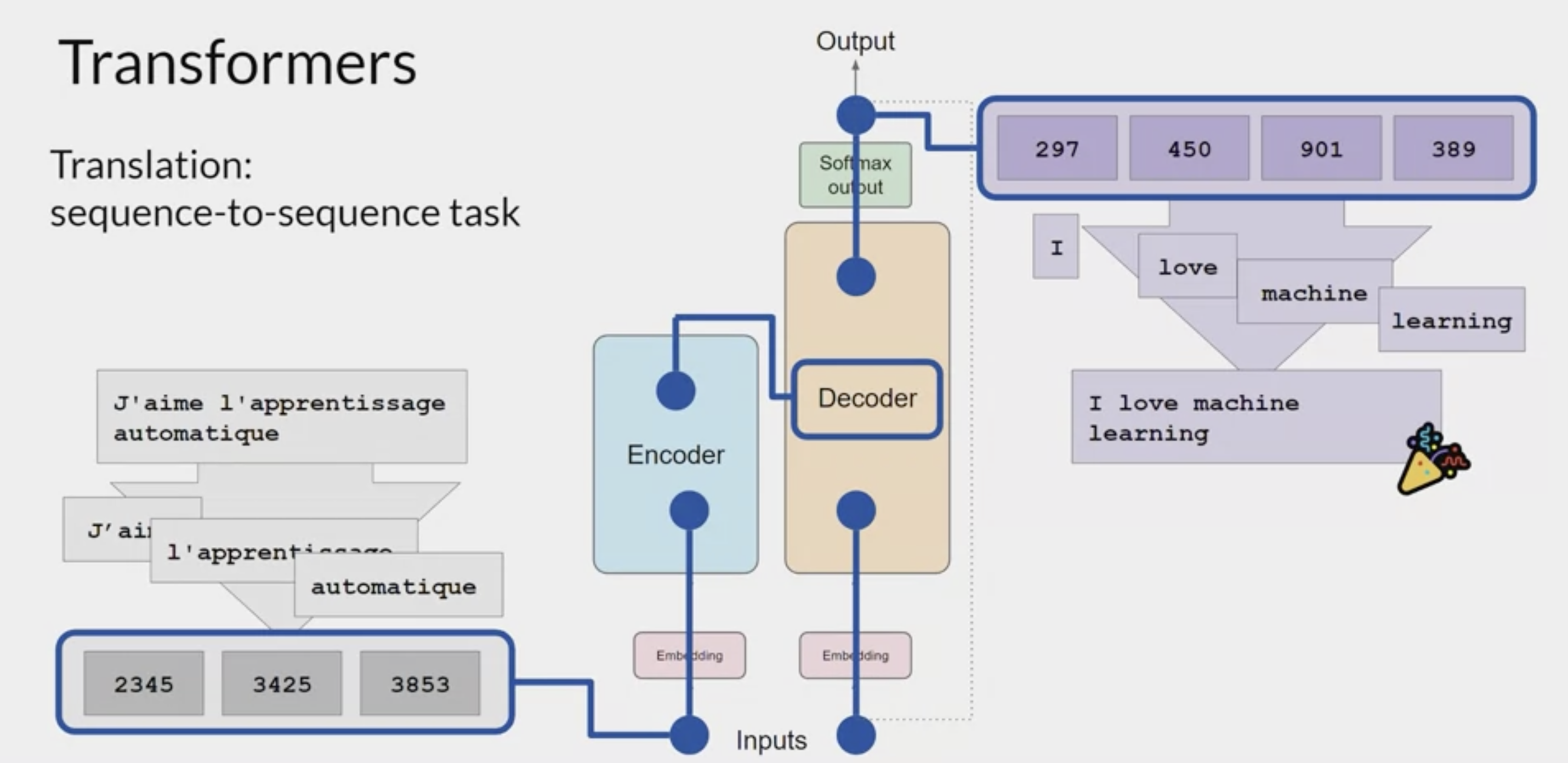
example: Generating text with transformers
- translation task
- a sequence-to-sequence task: the original objective of the transformer architecture designers.
- use a transformer model to translate the French phrase
[FOREIGN]into English.
Encoded side:
- First,
tokenize the input wordsusing this same tokenizer that was used to train the network. - These tokens are then added into the input on the encoder side of the network, passed through the embedding layer, and then fed into the
multi-headed attention layers. The outputs of the multi-headed attention layers are fed through a
feed-forward networkto the output of the encoder.- At this point, the data that leaves the encoder is a deep representation of the structure and meaning of the input sequence.
Decoded side:
- This representation is inserted into the middle of the decoder to influence the
decoder's self-attention mechanisms. - Next, a
start of sequence tokenis added to the input of the decoder. - This
triggers the decoder to predict the next token, based on the contextual understanding that it’s being provided from the encoder. The output of the decoder’s self-attention layers gets passed through the
decoder feed-forward networkand through a finalsoftmax output layer.At this point, we have our first token.
You’ll continue this loop, passing the output token back to the input to trigger the generation of the next token, until the model predicts an end-of-sequence token.
At this point, the final sequence of tokens can be detokenized into words, and you have the output.
- There are multiple ways in which you can use the output from the softmax layer to predict the next token. These can influence how creative you are generated text is.
Data preprocessing / embedding
Contextual data input
- Contextual data for LLM apps includes text documents, PDFs, and even structured formats like CSV or SQL tables.
- Data-loading and transformation solutions for this data vary widely across developers.
- Most use traditional ETL tools like
DatabricksorAirflow. - Some also use
document loadersbuilt into orchestration frameworks likeLangChain(powered by Unstructured) andLlamaIndex(powered by Llama Hub).
- Most use traditional ETL tools like
embeddings,
- most developers use the
OpenAI API, specifically with the text-embedding-ada-002 model. It’s easy to use (especially if you’re already already using other OpenAI APIs), gives reasonably good results, and is becoming increasingly cheap. - Some larger enterprises are also exploring
Cohere, which focuses their product efforts more narrowly on embeddings and has better performance in certain scenarios. - For developers who prefer open-source, the
Sentence Transformers libraryfromHugging Faceis a standard.
Vector Store
enable a fast and efficient kind of relevant search based on similarity.
- allow for fast searching of datasets and efficient identification of semantically related text.
important data storage strategy which contains vector representations of text.
a particularly useful data format for language models
internally they work with vector representations of language to generate text.
vector database
The most important piece of the preprocessing pipeline, from a systems standpoint
a particular implementation of a vector store where each vector is also identified by a key.
- This can allow the text generated by RAG to also include a citation for the document from which it was received.
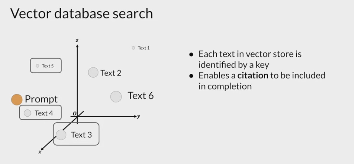
It’s responsible for efficiently storing, comparing, and retrieving up to billions of embeddings (i.e., vectors).
The most common choice is
Pinecone. It’s the default because it’s fully cloud-hosted, easy to get started with, and has many of the features larger enterprises need in production (e.g., good performance at scale, SSO, and uptime SLAs).Open source systemslike Weaviate, Vespa, and Qdrant: They generally give excellent single-node performance and can be tailored for specific applications, so they are popular with experienced AI teams who prefer to build bespoke platforms.Local vector management librarieslike Chroma and Faiss: They have great developer experience and are easy to spin up for small apps and dev experiments. They don’t necessarily substitute for a full database at scale.OLTP extensionslike pgvector: good solution for devs who see every database-shaped hole and try to insert Postgres, or enterprises who buy most of their data infrastructure from a single cloud provider. It’s not clear, in the long run, if it makes sense to tightly couple vector and scalar workloads.
Looking ahead, most of the open source vector database companies are developing cloud offerings. Our research suggests achieving strong performance in the cloud, across a broad design space of possible use cases, is a very hard problem. Therefore, the option set may not change massively in the near term, but it likely will change in the long term. The key question is whether vector databases will resemble their OLTP and OLAP counterparts, consolidating around one or two popular systems.
the embedding pipeline may become more important over time
- how embeddings and vector databases will evolve as the usable context window grows for most models.
- It’s tempting to say embeddings will become less relevant, because contextual data can just be dropped into the prompt directly.
- However, feedback from experts on this topic suggests the opposite, that the embedding pipeline may become more important over time. Large context windows are a powerful tool, but they also entail significant computational cost. So making efficient use of them becomes a priority.
- We may start to see different types of embedding models become popular, trained directly for model relevancy, and vector databases designed to enable and take advantage of this.
Prompt construction / retrieval
Strategies for prompting LLMs and incorporating contextual data are becoming increasingly complex—and increasingly important as a source of product differentiation.
Most developers start new projects by experimenting with simple prompts, consisting of direct instructions (
zero-shot prompting) or some example outputs (few-shot prompting).- These prompts often give good results but fall short of accuracy levels required for production deployments.
The next level of prompting
jiu jitsuis designed to ground model responses in some source of truth and provide external context the model wasn’t trained on.
advanced prompting strategies
- The Prompt Engineering Guide catalogs no fewer than 12 more advanced prompting strategies, including:
- chain-of-thought, self-consistency, generated knowledge, tree of thoughts, directional stimulus, and many others.
- These strategies can also be used in conjunction to support different LLM use cases like document question answering, chatbots, etc.
Orchestration frameworks
LangChainandLlamaIndexshine.workflow:
- They abstract away many of the details of prompt chaining;
- interfacing with external APIs (including determining when an API call is needed);
- retrieving contextual data from vector databases;
- and maintaining memory across multiple LLM calls.
- They also provide templates for many of the common applications mentioned above.
Their output is a prompt, or series of prompts, to submit to a language model. These frameworks are widely used among hobbyists and startups looking to get an app off the ground .
- LangChain is still a relatively new project (currently on version 0.0.201), but we’re already starting to see apps built with it moving into production.
Some developers, especially early adopters of LLMs, prefer to switch to raw Python in production to eliminate an added dependency. But we expect this DIY approach to decline over time for most use cases, in a similar way to the traditional web app stack.
- ChatGPT.
- In its normal incarnation, ChatGPT is an app, not a developer tool. But it can also be accessed as an API.
- it performs some of the same functions as other orchestration frameworks, such as: abstracting away the need for bespoke prompts; maintaining state; and retrieving contextual data via plugins, APIs, or other sources.
- While not a direct competitor to the other tools listed here, ChatGPT can be considered a substitute solution, and it may eventually become a viable, simple alternative to prompt construction.
Prompt execution / inference
Prompt execution / inference
OpenAI- Today, OpenAI is the leader among language models. Nearly every developer starts new LLM apps using the OpenAI API with the gpt-4 or gpt-4-32k model.
- This gives a best-case scenario for app performance and is easy to use, in that it operates on a wide range of input domains and usually requires no fine-tuning or self-hosting.
When projects go into production and start to scale, a broader set of options come:
Switching to gpt-3.5-turbo: It’s ~50x cheaper and significantly faster than GPT-4. Many apps don’t need GPT-4-level accuracy, but do require low latency inference and cost effective support for free users.Other proprietary vendors (like Anthropic’s Claude models): Claude offers fast inference, GPT-3.5-level accuracy, more customization options for large customers, and up to a 100k context window (though we’ve found accuracy degrades with the length of input).Triaging requests to open source models: This can be especially effective in high-volume B2C use cases like search or chat, where there’s wide variance in query complexity and a need to serve free users cheaply.conjunction with fine-tuning open source base models, platforms like Databricks, Anyscale, Mosaic, Modal, and RunPod are used by a growing number of engineering teams.
A variety of inference options are available for open source models, including simple API interfaces from Hugging Face and Replicate; raw compute resources from the major cloud providers; and more opinionated cloud offerings like those listed above.
Open-source modelstrailproprietary offerings, but the gap is starting to close.The LLaMa models from Meta
- set a new bar for open source accuracy and kicked off a flurry of variants.
- Since LLaMa was licensed for research use only, a number of new providers have stepped in to train alternative base models (e.g., Together, Mosaic, Falcon, Mistral).
Meta is also debating a truly open source release of LLaMa2.
- When open source LLMs reach accuracy levels comparable to GPT-3.5, we expect to see a Stable Diffusion-like moment for text—including massive experimentation, sharing, and productionizing of fine-tuned models.
Hosting companies like Replicate are already adding tooling to make these models easier for software developers to consume. There’s a growing belief among developers that smaller, fine-tuned models can reach state-of-the-art accuracy in narrow use cases.
Most developers haven’t gone deep on operational tooling for LLMs yet.
- Caching is relatively common—usually based on Redis—because it improves application response times and cost.
- Tools like Weights & Biases and MLflow (ported from traditional machine learning) or PromptLayer and Helicone (purpose-built for LLMs) are also fairly widely used. They can log, track, and evaluate LLM outputs, usually for the purpose of improving prompt construction, tuning pipelines, or selecting models.
- There are also a number of new tools being developed to validate LLM outputs (e.g., Guardrails) or detect prompt injection attacks (e.g., Rebuff). Most of these operational tools encourage use of their own Python clients to make LLM calls, so it will be interesting to see how these solutions coexist over time.
the static portions of LLM apps (i.e. everything other than the model) also need to be hosted somewhere.
- The most common solutions we’ve seen so far are standard options like Vercel or the major cloud providers.
- Startups like Steamship provide end-to-end hosting for LLM apps, including orchestration (LangChain), multi-tenant data contexts, async tasks, vector storage, and key management.
- And companies like Anyscale and Modal allow developers to host models and Python code in one place.
AI agents frameworks
AutoGPT, described as “an experimental open-source attempt to make GPT-4 fully autonomous,”The in-context learning pattern is effective at solving hallucination and data-freshness problems, in order to better support content-generation tasks.
Agents, on the other hand, give AI apps a fundamentally new set of capabilities: to solve complex problems, to act on the outside world, and to learn from experience post-deployment.
- They do this through a combination of
advanced reasoning/planning, tool usage, and memory / recursion / self-reflection.
- They do this through a combination of
agents have the potential to become a central piece of the LLM app architecture
And existing frameworks like LangChain have incorporated some agent concepts already. There’s only one problem: agents don’t really work yet. Most agent frameworks today are in the proof-of-concept phase—capable of incredible demos but not yet reliable, reproducible task-completion.
LLM Tools
Medusa
Our approach revisits an underrated gem from the paper “Blockwise Parallel Decoding for Deep Autoregressive Models” [Stern et al. 2018] back to the invention of the Transformer model. rather than pulling in an entirely new draft model to predict subsequent tokens, why not simply extend the original model itself? This is where the “Medusa heads” come in.
a simpler, user-friendly framework for accelerating LLM generation.
Instead of using an additional draft model like
speculative decoding, Medusa merely introduces a few additional decoding heads, following the idea of [Stern et al. 2018] with some other ingredients.Despite its simple design, Medusa can improve the generation efficiency of LLMs by about 2x.
These additional decoding heads seamlessly integrate with the original model, producing blocks of tokens at each generative juncture.
benefit:
Unlike the draft model, Medusa heads can be trained in conjunction with the original model (which remains frozen during training). This method allows for
fine-tuning large models on a single GPU, taking advantage of the powerful base model’s learned representations.also, since the new heads consist of just a single layer akin 类似的 to the original language model head, Medusa does not add complexity to the serving system design and is friendly to distributed settings.
On its own, Medusa heads don’t quite hit the mark of doubling processing speeds. But here’s the twist:
When we pair this with a tree-based attention mechanism, we can verify several candidates generated by Medusa heads in parallel. This way, the Medusa heads’ predictive prowess truly shone through, offering a 2x to 3x boost in speed.
Eschewing the traditional importance sampling scheme, we created an efficient and high-quality alternative crafted specifically for the generation with Medusa heads. This new approach entirely sidesteps the sampling overhead, even adding an extra pep to Medusa’s already accelerated step.
In a nutshell, we solve the challenges of speculative decoding with a simple system:
No separate model: Instead of introducing a new draft model, train multiple decoding heads on the same model.
Simple integration to existing systems: The training is parameter-efficient so that even GPU poor can do it. And since there is no additional model, there is no need to adjust the distributed computing setup.
Treat sampling as a relaxation 放松: Relaxing the requirement of matching the distribution of the original model makes the non-greedy generation even faster than greedy decoding.
The figure below offers a visual breakdown of the Medusa pipeline for those curious about the nuts and bolts.
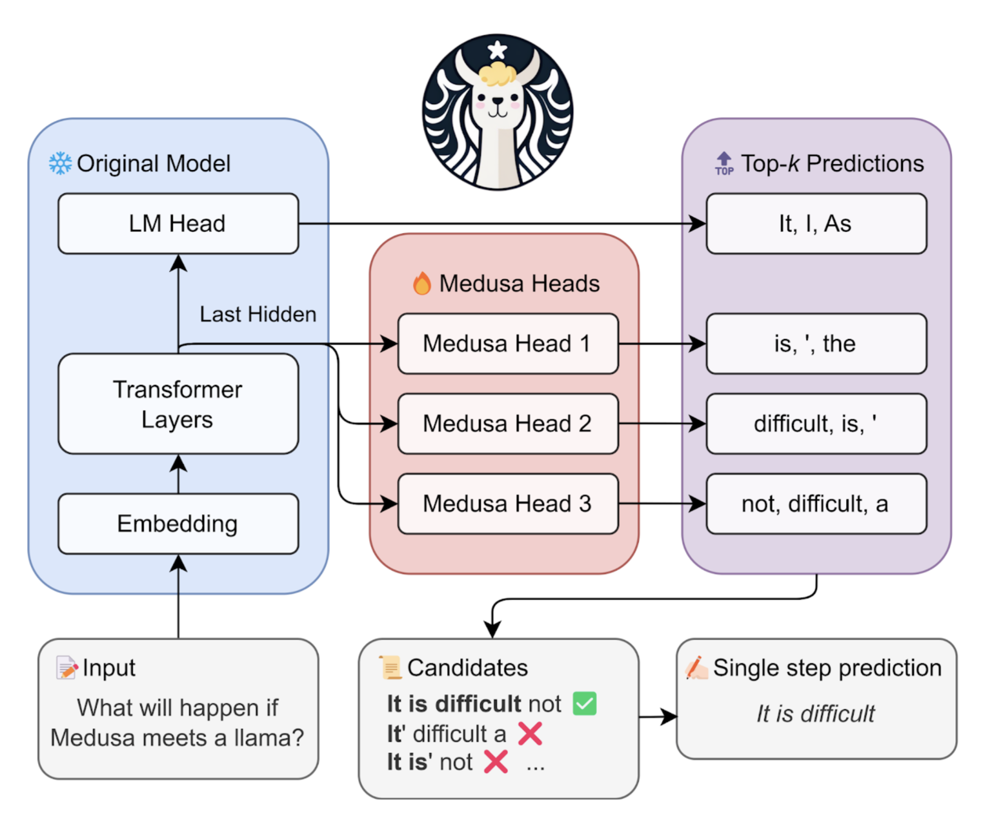
Overview of Medusa
Medusa introduces
multiple headson top of the last hidden states of the LLM, enabling the prediction of several subsequent tokens in parallel.When augmenting a model with Medusa heads, the original model is frozen during training, and only the Medusa heads undergo fine-tuning. This approach makes it feasible to
fine-tune large models on a single GPU.During inference, each head generates multiple top predictions for its designated position. These predictions are assembled into candidates and processed in parallel using a
tree-based attention mechanism.The final step involves utilizing a typical acceptance scheme to select reasonable continuations, and the longest accepted candidate prefix will be used for the next decoding phase.
The efficiency of the decoding process is enhanced by accepting more tokens simultaneously, thus reducing the number of required decoding steps.
Let’s dive into the three components of Medusa: Medusa heads, tree attention, and typical acceptance scheme.
Medusa heads
akin to the language model head in the original architecture (the last layer of a causal Transformer model), but with a twist:
- they predict multiple forthcoming tokens, not just the immediate next one. Drawing inspiration from the Blockwise Parallel Decoding approach, we implement each Medusa head as a single layer of feed-forward network, augmented with a residual connection.
Training these heads is remarkably straightforward. either use the same corpus 本体 that trained the original model or generate a new corpus using the model itself.
Importantly, during this training phase, the original model remains static; only the Medusa heads are fine-tuned.
This targeted training results in a highly parameter-efficient process that reaches convergence 趋同 swiftly 迅速地, especially when compared to the computational heaviness 沉重 of training a separate draft model in speculative decoding methods.
The efficacy of Medusa heads is quite impressive. Medusa heads achieve a top-1 accuracy rate of approximately 60% for predicting the ‘next-next’ token.
Tree attention
During our tests, we uncovered some striking metrics: although the top-1 accuracy for predicting the ‘next-next’ token hovers around 60%, the top-5 accuracy soars to over 80%.
This substantial increase indicates that if we can strategically leverage the multiple top-ranked predictions made by the Medusa heads, we can significantly amplify the number of tokens generated per decoding step.
With this goal, we first craft a set of candidates by taking the Cartesian product of the top predictions from each Medusa head.
We then encode the dependency graph into the attention following the idea from graph neural networks so that we can process multiple candidates in parallel.
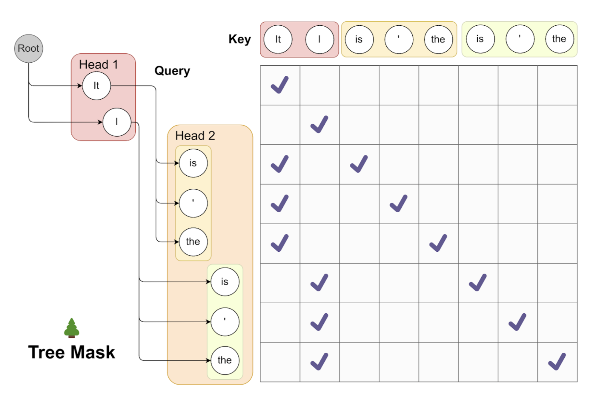
Tree Attention. This visualization demonstrates the use of tree attention to process multiple candidates concurrently.
As exemplified, the top-2 predictions from the first Medusa head and the top-3 from the second result in 2*3=6 candidates. Each of these candidates corresponds to a distinct branch within the tree structure.
To guarantee that each token only accesses its predecessors, we devise an attention mask that exclusively permits attention flow from the current token back to its antecedent tokens. The positional indices for positional encoding are adjusted in line with this structure.
For example, let’s consider a scenario where we use top-2 predictions from the first Medusa head and top-3 predictions from the second
- In this case, any prediction from the first head could be paired with any prediction from the second head, culminating in a multi-level tree structure.
- Each level of this tree corresponds to predictions from one of the Medusa heads. Within this tree, we implement an attention mask that restricts attention only to a token’s predecessors, preserving the concept of historical context.
- By doing so and by setting positional indices for positional encoding accordingly, we can process a wide array of candidates simultaneously without needing to inflate the batch size.
We would also remark that a few independent works also adopt very similar ideas of tree attention [1, 2]. Compared with them, our methodology leans towards a simpler form of tree attention where the tree pattern is regular and fixed during inference, which enables a preprocessing of tree attention mask that further improves the efficiency.
Typical acceptance
- In earlier research on speculative decoding, the technique of importance sampling was used to generate diverse outputs closely aligned with the original model’s predictions.
- However, later studies showed that this method tends to become less efficient as you turn up the “creativity dial,” known as the sampling temperature.
In simpler terms, if the draft model is just as good as the original model, you should ideally accept all its outputs, making the process super efficient. However, importance sampling will likely reject this solution in the middle.
In the real world, we often tweak the sampling temperature just to control the model’s creativity, not necessarily to match the original model’s distribution. So why not focus on just accepting plausible 貌似合理的 candidates?
We then introduce the typical acceptance scheme.
Drawing inspiration from existing work on truncation 缩短 sampling, we aim to pick candidates that are likely enough according to the original model. We set a threshold based on the original model’s prediction probabilities, and if a candidate exceeds this, it’s accepted.
- In technical jargon, we take the minimum of a hard threshold and an entropy 熵, dependent threshold to decide whether to accept a candidate as in truncation sampling.
- This ensures that meaningful tokens and reasonable continuations are chosen during decoding.
- We always accept the first token using greedy decoding, ensuring that at least one token is generated in each step.
- The final output is then the longest sequence that passes our acceptance test.
What’s great about this approach is its adaptability.
If set the sampling temperature to zero, it simply reverts to the most efficient form, greedy decoding.
When you increase the temperature, our method becomes even more efficient, allowing for longer accepted sequences, a claim we’ve confirmed through rigorous testing.
in essence, our typical acceptance scheme offers a more efficient way to generate the creative output of LLMs.
accelerate models
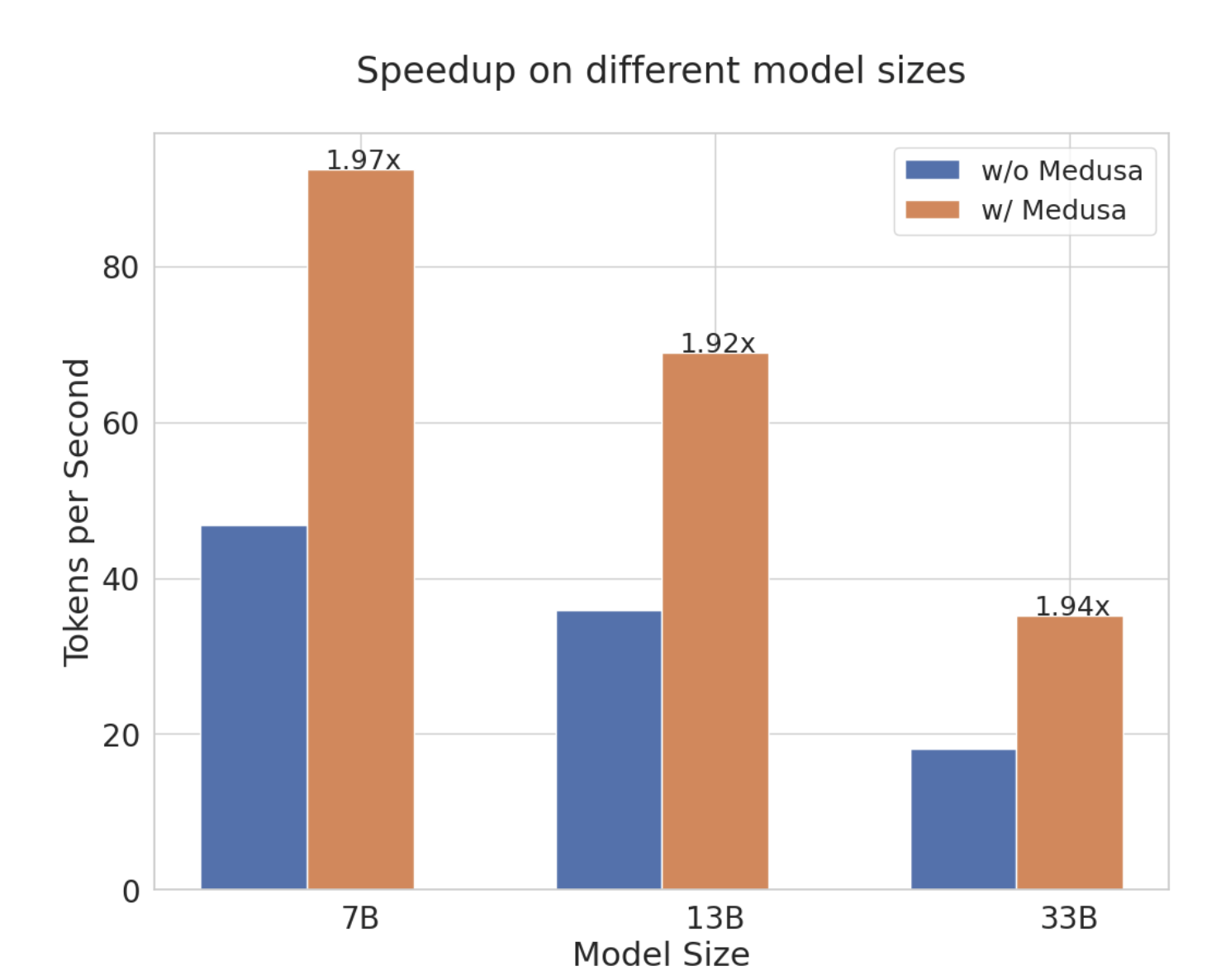
We tested Medusa with Vicuna models (specialized Llama models fine-tuned specifically for chat applications).
- These models vary in size, with parameter counts of 7B, 13B, and 33B.
- Our goal was to measure how Medusa could accelerate 加速 these models in a real-world chatbot environment.
When it comes to training Medusa heads, we opted for a simple approach. We utilized the publicly available ShareGPT dataset, a subset of the training data originally used for Vicuna models and only trained for a single epoch.
this entire training process could be completed in just a few hours to a day, depending on the model size, all on a single A100-80G GPU.
Notably, Medusa can be easily combined with a quantized base model to reduce the memory requirement. We take this advantage and use an 8-bit quantization 量化 when training the 33B model.
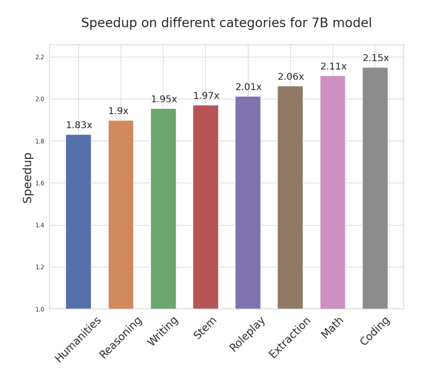
To simulate a real-world setting, we use the MT bench for evaluation. The results were encouraging: With its simple design, Medusa consistently achieved approximately a 2x speedup in wall time across a broad spectrum of use cases.
Remarkably, with Medusa’s optimization, a 33B parameter Vicuna model could operate as swiftly as a 13B model.
Ablation Study 消融研究
When harnessing the predictive abilities of Medusa heads, we enjoy the flexibility to select how many top candidates each head should consider.
- For instance, we might opt for the top-3 predictions from the first head and the top-2 from the second. When we take the Cartesian product of these top candidates, we generate a set of six continuations for the model to evaluate.
- This level of configurability comes with its trade-offs.
- On the one hand, selecting more top predictions increases the likelihood of the model accepting generated tokens.
On the other, it also raises the computational overhead at each decoding step. To find the optimal balance, we experimented with various configurations and identified the most effective setup, as illustrated in the accompanying figure.
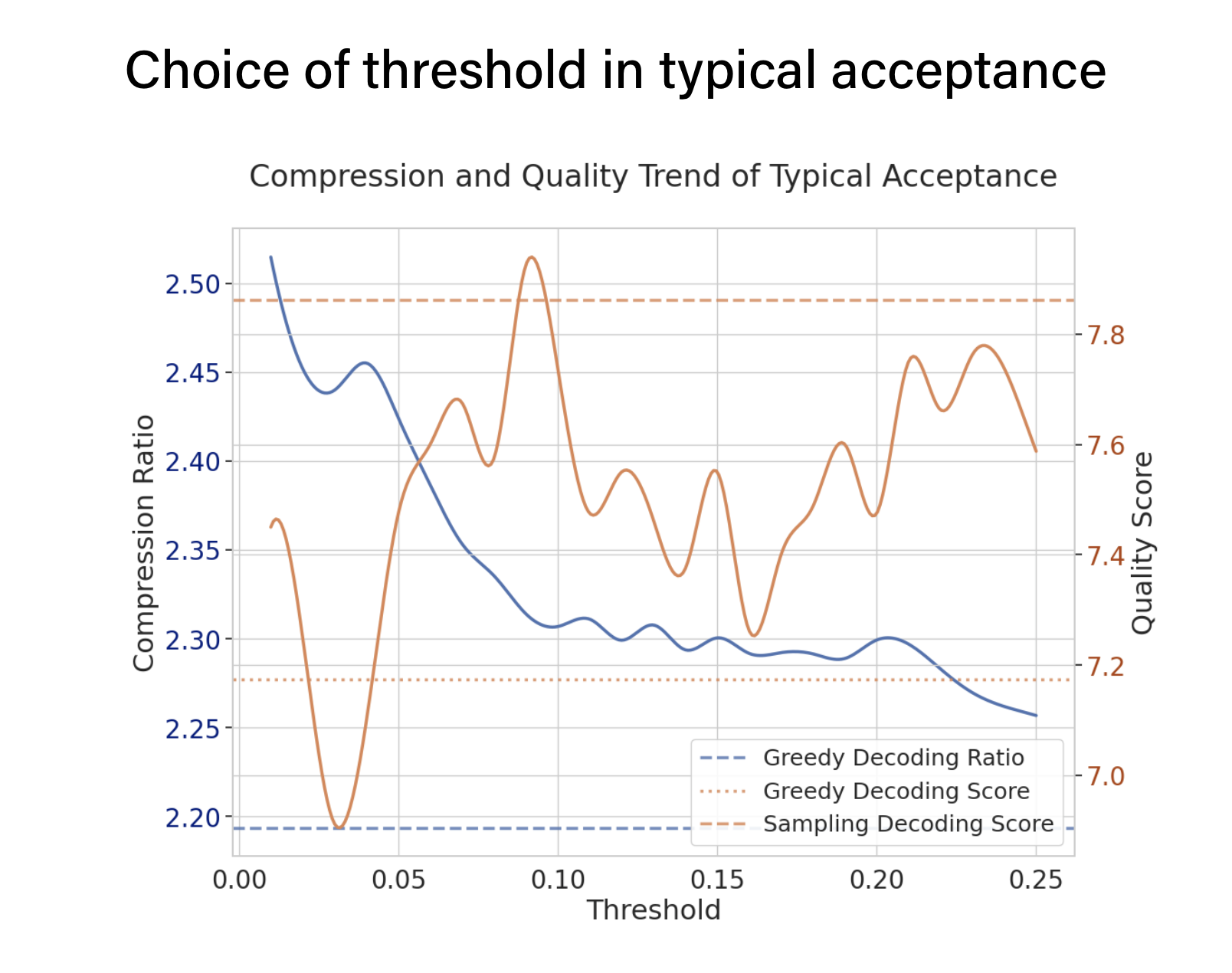
- In the typical acceptance scheme, a critical hyperparameter—referred to as the
‘threshold’: whether the tokens generated are plausible based on the model’s own predictions. The higher this threshold, the more stringent the criteria for acceptance, which in turn impacts the overall speedup gained through this approach.
- We explore this trade-off between quality and speedup through experiments on two creativity-oriented tasks from the MT bench. The results, depicted in the figure, reveal that the typical acceptance offers a 10% speedup compared to greedy decoding methods. This speedup is notably better than when employing speculative decoding with random sampling, which actually slowed down the process compared to greedy decoding.
LLM Pre-Training
[./LLM/2023-04-24-LLM_Pretraining.md]
LLM Data Training
[./LLM/2023-04-24-LLM_DataTraining.md]
Confidence score for ML model
[./LLM/2023-04-24-LLM_ConfidenceScore.md]
Transparency
Transparency in the context of AI models refers to the degree to which the inner workings of the model are understandable, interpretable, and explainable to humans. It encompasses several aspects:
- Explainability:
- This refers to the ability to understand and interpret the model’s decisions.
- An interpretable model
provides clear and understandable reasonsfor its predictions or actions. - This is crucial, especially in high-stakes applications like healthcare or finance, where accountability and trust are essential.
- Visibility:
- Transparency also involves making the model architecture, parameters, and training data visible to those who are affected by its decisions.
- This allows external parties to scrutinize the model for biases, ethical concerns, or potential risks.
- Audibility:
- The ability to audit an AI model involves examining its processes, inputs, and outputs to ensure it aligns with ethical and legal standards.
- Auditing enhances accountability and helps identify and rectify issues or biases.
- Comprehensibility:
- A transparent AI model should be comprehensible to various stakeholders, including domain experts, policymakers, and the general public. This involves presenting complex technical concepts in a way that is accessible to non-experts.
- Fairness and Bias: Transparency also relates to addressing biases in AI models. Understanding how the model makes decisions can help identify and rectify biased behavior, ensuring fair treatment across diverse demographic groups.
- Transparency is crucial for building trust in AI systems, especially as they are increasingly integrated into various aspects of society. It helps users, regulators, and the general public understand how AI systems function, assess their reliability, and hold developers and organizations accountable for their impact. Various techniques and tools are being developed to enhance the transparency of AI models, but it remains an ongoing area of research and development.
The Foundation Model Transparency Index
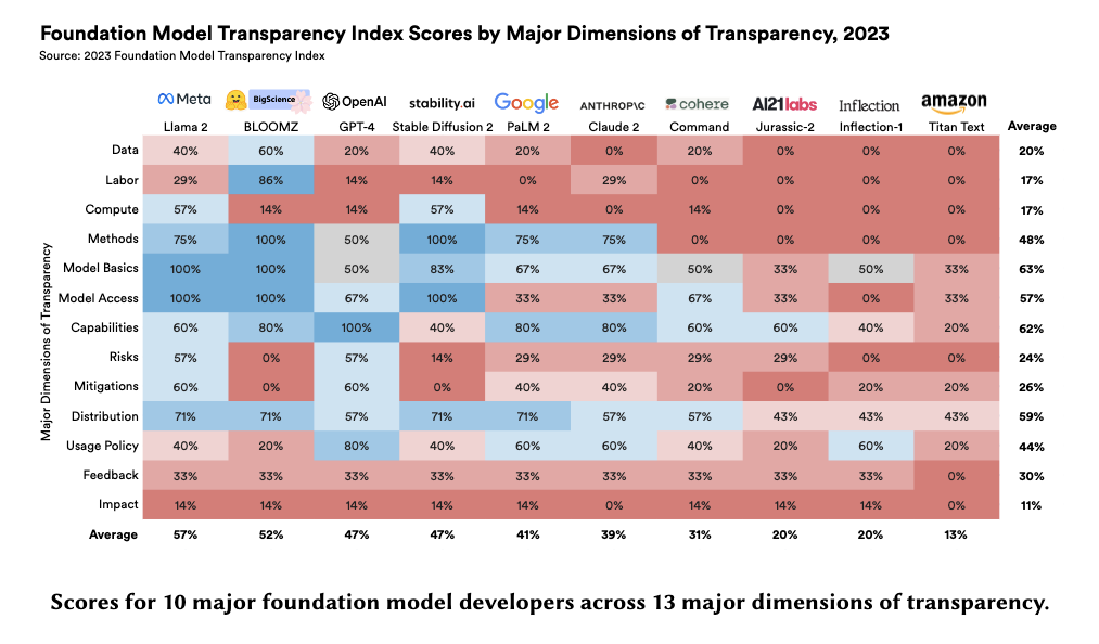
The Foundation Model Transparency Index 3.
Foundation models have rapidly permeated society, catalyzing a wave of generative AI applications spanning enterprise and consumer-facing contexts.
While the societal impact of foundation models is growing, transparency is on the decline, mirroring the opacity that has plagued past digital technologies (e.g. social media).
Reversing this trend is essential:
- transparency is a vital precondition for public accountability, scientific innovation, and effective governance. To assess the transparency of the founda- tion model ecosystem and help improve transparency over time, we introduce the Foundation Model Transparency Index. The 2023 Foundation Model Transparency Index specifies 100 fine-grained indicators that comprehensively codify transparency for foundation models, spanning the upstream resources used to build a foundation model (e.g. data, labor, compute), details about the model itself (e.g. size, capabilities, risks), and the downstream use (e.g. distribution channels, usage policies, affected geographies). We score 10 major foundation model developers (e.g. OpenAI, Google, Meta) against the 100 indicators to assess their transparency. To facilitate and standardize assessment, we score developers in relation to their practices for their flagship foundation model (e.g. GPT-4 for OpenAI, PaLM 2 for Google, Llama 2 for Meta). We present 10 top-level findings about the foundation model ecosystem: for example, no developer currently discloses significant information about the downstream impact of its flagship model, such as the number of users, affected market sectors, or how users can seek redress for harm. Overall, the Foundation Model Transparency Index establishes the level of transparency today to drive progress on foundation model governance via industry standards and regulatory intervention.
GenAI for Code
Pretrained transformer-based modelshave shown high performance innatural language generationtask. However, a new wave of interest has surged:automatic programming language generation.This task consists of translating natural language instructions to a programming code. effort is still needed in automatic code generation
When developing software, programmers use both
natural language (NL)andprogramming language (PL).- natural language is used to write documentation (ex: JavaDoc) to describe different classes, methods and variables.
- Documentation is usually written by experts and aims to provide a comprehensive explanation of the source code to every person who wants to use/develop the project.
the automation of
programming code generationfrom natural language has been studied using various techniques of artificial intelligence (AI): automatically generate code for simple tasks, while allowing them to tackle only the most difficult ones.After the big success of Transformers Neural Network, it has been adapted to many
Natural Language Processing (NLP) tasks(such as question answering, text translation, automatic summarization)- popular models are GPT, BERT, BART, and T5
One of the main factors of success: trained on very large corpora.
Recently, there has been an increasing interest in programming code generation. scientific community based its research on proposing systems that are based on pretrained transformers.
CodeGPTandGPT-adaptedare based onGPT2PLBARTis based onBART,CoTexTfollowsT5.- Note that these models have been pretrained on
bimodal data(containing both PL and NL) and onunimodal data(containing only PL).
Programming language generation is more challenging than standard text generation, PLs contain stricter grammar and syntactic rules.
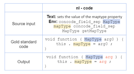
an example of an input sequence received by the model (in NL), the output of the model (in PL) and the target code (called gold standard or reference code).
study from the state of the art:
initialize the model from powerful pretrained models, instead of performing a training from scratch.
- Models initialized from previous pretrained weights achieve better performance than models trained from scratch
additional pretraining
Transformers neural network improves its performance significantly from increasing the amount of pretraining datafor some specific tasks, the way to improve the model’s performance is to
pretrain it with a dataset that belongs to a specific domain,- Models such as
SciBERTandBioBERThave shown the benefits to pretrain a model using data related to a specific domain.
- Models such as
Increased data implies better training performance. This finding is intuitive since a large and diversified dataset helps improving the model’s representation.
The objective learning used during the pretraining stage gives the model some benefits when learning the downstream tasks
a low number of epochs when pretraining a model leads to higher scores in generation tasks.
scale the input and output length during the fine-tuning of the model
The input and output sequence length used to train the model matters in the performance of the model
Number of steps, when increased the length of sequences in the model, it increased the number of fine-tuning steps. a way to improve the model’s performance is by increasing the number of steps in the training.
carry out experiments combining the unimodal and bimodal data in the training
T5 has shown the best performance in language generation tasks.
Fine-tuning
additional pretraining
dataset
CONCODE- contains context of a real world Java programming environment.
- aims to generate Java member functions that have class member variables from documentation.
CONCODEdataset: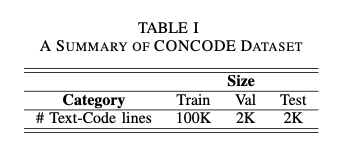
CodeSearchNet, Corpus, and GitHub Repositories.
EXPERIMENTAL
Evaluation Metrics
To evaluate the models
BLEU:a metric based on
n-gram precisioncomputed between the candidate and the reference(s).N-gram precisionpenalizes the model if:- (1) words appear in the candidate but not in any of the references, or
- (2) word appear more times in the candidate than in the maximum reference count.
- However, the metric fails if the candidate does not have the appropriate length.
- we use the
corpus-level BLEU scorein the code generation task.
CodeBLEU:- works via
n-grammatch, and it takes into account both the syntactic and semantic matches. - The syntax match is obtained by matching between the
code candidate and code reference(s) sub-treesofabstract syntax tree (AST). - The semantic match considers the data-flow structure.
- works via
Exact Match (EM):- the ratio of the number of predictions that match exactly any of the code reference(s).
usage
Juptyper
To run a shell command from within a notebook cell, you must put a ! in front of the command: !pip install hyperopt
1
2
3
4
5
6
7
8
9
10
11
12
13
14
15
16
17
18
19
20
21
22
23
24
25
26
27
28
29
30
31
32
33
34
!nvidia-smi --list-gpus


!pip install --upgrade pip

!pip uninstall -y git+https://github.com/openai/CLIP.git \
  urllib3==1.25.10 \
  sentence_transformers \
  torch torchvision pytorch-lightning lightning-bolts

# install supporting puthon packages for Data Frame processing
# and for Progress Bar
!pip install numpy pandas matplotlib tqdm scikit-learn

# install only the older version of Torch
!pip install --ignore-installed \
    urllib3==1.25.10 \
    torch torchvision pytorch-lightning lightning-bolts

# install latest (Upgrade) sentence transformers for fine-tuning
!pip install --ignore-installed \
  urllib3==1.25.10 \
  pyyaml \
  sentence_transformers

# Use CLIP model from OpenAI
!pip install git+https://github.com/openai/CLIP.git

# load the python package to run Pandas in parallel for better speed
!pip install pandarallel

!pip install torchaudio

!pip uninstall -y nvidia_cublas_cu11
Hugging Face
like github repo
- search for an AI model
1
2
3
4
5
6
7
8
9
10
11
12
13
14
15
16
17
18
19
20
21
22
23
24
25
26
27
28
# +++++ Getting started with our git and git-lfs interface
# If you need to create a repo from the command line (skip if you created a repo from the website)
pip install huggingface_hub
# You already have it if you installed transformers or datasets
huggingface-cli login
# Log in using a token from huggingface.co/settings/tokens
# Create a model or dataset repo from the CLI if needed
huggingface-cli repo create repo_name --type {model, dataset, space}


# +++++ Clone the model or dataset locally
# Make sure you have git-lfs installed
# (https://git-lfs.github.com)
git lfs install
git clone https://huggingface.co/username/repo_name


# +++++ Then add, commit and push any file you want, including larges files
# save files via `.save_pretrained()` or move them here
git add .
git commit -m "commit from $USER"
git push


# +++++ In most cases, if you're using one of the compatible libraries, the repo will then be accessible from code, through its identifier: username/repo_name
# For example for a transformers model, anyone can load it with:
tokenizer = AutoTokenizer.from_pretrained("username/repo_name")
model = AutoModel.from_pretrained("username/repo_name")
Generative AI Time Series Forecasting
Multivariate Time Series Forecasting
Generative AI Transformers for Time Series Forecasting
Falcon 40b
Chatgpt competitor - https://huggingface.co/tiiuae/falcon-40b
Power of Falcon 40b chat - https://huggingface.co/spaces/HuggingFaceH4/falcon-chat
Pre-Training - https://huggingface.co/tiiuae/falcon-40b#training-data
or https://github.com/aws-samples/amazon-sagemaker-generativeai/blob/main/studio-notebook-fine-tuning/falcon-40b-qlora-finetune-summarize.ipynb
Chat with Falcon-40B-Instruct, brainstorm ideas, discuss the holiday plans, and more!
- ✨ This demo is powered by Falcon-40B, finetuned on the Baize dataset, and running with Text Generation Inference. Falcon-40B is a state-of-the-art
large language modelbuilt by the Technology Innovation Institute in Abu Dhabi. It is trained on 1 trillion tokens (including RefinedWeb) and available under the Apache 2.0 license. It currently holds the 🥇 1st place on the 🤗 Open LLM leaderboard. This demo is made available by the HuggingFace H4 team. - 🧪 This is only a first experimental preview: the H4 team intends to provide increasingly capable versions of Falcon Chat in the future, based on improved datasets and RLHF/RLAIF.
- 👀 Learn more about Falcon LLM:
falconllm.tii.ae - ➡️️ Intended Use: this demo is intended to showcase an early finetuning of Falcon-40B, to illustrate the impact (and limitations) of finetuning on a dataset of conversations and instructions. We encourage the community to further build upon the base model, and to create even better instruct/chat versions!
- ⚠️ Limitations: the model can and will produce factually incorrect information, hallucinating facts and actions. As it has not undergone any advanced tuning/alignment, it can produce problematic outputs, especially if prompted to do so. Finally, this demo is limited to a session length of about 1,000 words.
CodeParrot
TAPEX
Give a table of data and then query
- 0 shot question (answer right away)
- fine tune: https://github.com/SibilTaram/tapax_transformers/tree/add_tapex_bis/examples
- demo: https://huggingface.co/microsoft/tapex-base
common LLM
GPT
- the greatest achievement in this field as it amassed 100 million active users in 2 months from the day of its release.
- ChatGPT
- GPT-4 by OpenAI 🔥
- programming code generation
CodeGPTandGPT-adaptedbased on GPT2CodeGPTis trained from scratch onCodeSearchNetdatasetCodeGPT-adaptedis initialized from GPT-2 pretrained weights.
LLaMA
- by Meta 🦙
AlexaTM
- by Amazon 🏫
Minerva
- by Google ✖️➕
BERT
- programming code generation:
CodeBERT SciBERT,BioBERT
BART
- programming code generation
PLBARTis based onBART,PLBARTuses the same architecture thanBARTbase.PLBARTuses three noising strategies: token masking, token deletion and token infilling.
T5
- programming code generation
CoTexTfollowsT5: based their pretraining onCodeSearchNet
JaCoText
- model based on Transformers neural network.
- pretrained model based on Transformers
- It aims to generate java source code from natural language text.
1 GPT 系列(OpenAI)
语言模型
- 语言模型是 GPT 系列模型的基座。[^通俗易懂的LLM(上篇)]
语言模型,
- 简单来说,就是看一个句子是人话的可能性。
专业一点来说
- 给定一个句子,其字符是 $W=(w_{1},w_{2},\cdots,w_{L})$
那么,从语言模型来看,这个句子是人话的可能性就是: $\begin{aligned} P(W)&=P(w_{1},w_{2},\cdots,w_{L})\ &=P(w_{1})P(w_{2} w_{1})P(w_{3} w_{1},w_{2})\cdots P(w_{L} w_{1},w_{2},\cdots,w_{L-1})\ \end{aligned}$ 但是, $L$ 太长就会很稀疏,直接算这个概率不好计算,我们就可以用近似计算: $\begin{aligned} P(W)&=P(w_{1},w_{2},\cdots,w_{L})\ &=P(w_{1})P(w_{2} w_{1})P(w_{3} w_{1},w_{2})\cdots P(w_{L} w_{1},w_{2},\cdots,w_{L-1})\ &=P(w_{1})P(w_{2} w_{1})\cdots P(w_{L} w_{L-N},\cdots,w_{L-1}) \end{aligned}$ - 这就是常说的 N-gram 统计语言模型,N 通常是 2,3,4。
- 特别的,当
N=1时,语言模型就退化为各个字符出现的概率之积。 - 当
N=4时语言模型就比较大了,实际应用中一般最大也就是 4 了。 根据条件概率 $P(w_{L} w_{L-N},\cdots,w_{L-1})$,我们就能知道给定前 N 个字,下一个字是什么字的概率了。
语言模型的评价指标可以采用 PPL(困惑度,Perplexity [^语言模型])
1.1 GPT-1, GPT-2, GPT-3
2017 年,
Google推出Transformer,利用 attention 完全替代过往深度学习中的 Recurrence 和 Convolution 结构,直白地展现出了“大一统模型”的野心,”xxx is all you need”也成了一个玩不烂的梗。- 2018 年 6 月,
OpenAI推出基于Transformer Decoder改造的第一代GPT(Generative Pre-Training),有效证明了在 NLP 领域上使用预训练+微调方式的有效性。 2018 年 10 月,
Google推出基于Transformer Encoder部分的Bert,在同样参数大小的前提下,其效果领跑于 GPT-1,一时成为 NLP 领域的领头羊。不甘示弱的 OpenAI 在 4 个月后,推出更大的模型GPT-2(GPT-1: 110M,Bert: 340M,GPT-2: 1.5B),同时,OpenAI 也知道,光靠增加模型大小和训练数据集来获得一个和 Bert 差不多效果的模型,其实是没有技术含量的。于是,在 GPT-2 里,OpenAI 引入 zero-shot 并证明了其有效性。
- 此后,OpenAI 在 LLM 上义无反顾地走了下去,在 2020 年 6 月推出巨人 GPT-3,参数量高达 175B,各类实验效果达到顶峰,据说一次训练费用为 1200w 美元,“贵”也成了普通工业界踏足 GPT 系列的壁垒之一。
GPT-1
- GPT-1 是 OpenAI 在论文《Improving Language Understanding by Generative Pre-Training》中提出的生成式预训练语言模型。
该模型的核心思想: 通过二段式的训练
- 第一个阶段是利用语言模型进行预训练(无监督形式)
- 第二阶段通过 Fine-Tuning 的模式解决下游任务(监督模式下 GPT-1 可以很好地完成若干下游任务,包括文本分类, 自然语言推理, 问答, 语义相似度等。
在多个下游任务中,微调后的 GPT-1 性能均超过了当时针对特定任务训练的 SOTA 模型。
自然语言推理(Natural Language Inference 或者 Textual Entailment): 判断两个句子是包含关系(entailment),矛盾关系(contradiction),或者中立关系(neutral);
问答和常识推理(Question answering and commonsense reasoning): 类似于多选题,输入一个文章,一个问题以及若干个候选答案,输出为每个答案的预测概率;
语义相似度(Semantic Similarity): 判断两个句子是否语义上是相关的;
- 分类(Classification): 判断输入文本是指定的哪个类别。
GPT-1 的模型结构及训练流程。
模型结构:
GPT-1 基础架构是基于
Transformer的Decoder部分,同时删除了Encoder-Decoder Attention层,只保留了Masked Multi-Head Attention层和Feed Forward层。Transformer 结构提出之始便用于机器翻译任务
- 机器翻译是一个序列到序列的任务,因此 Transformer 设计了
- Encoder 用于提取源端语言的语义特征
- Decoder 提取目标端语言的语义特征,并生成相对应的译文。
GPT-1 目标是服务于单序列文本的生成式任务,所以含弃了关于 Encoder 部分,包括 Decoder 的 Encoder-Decoder Attention 层。
整体是 12 层的 Transformer-Decoder 变体,如下图所示:

- 除此之外,GPT-1 还将 attention 的维数扩大到 768(原来为 512),将 attention 的头数增加到 12 个(原来为 8 个),将 Feed Forward 层的隐层维数增加到 3072(原来为 2048),总参数达到 110M。
- GPT-1 还优化了学习率预热算法,使用更大的 BPE 码表(词表大小为 40478,478 个 base characters + 40000 个结合的字符),激活函数 ReLU 改为对梯度更新更友好的高斯误差线性单元 GeLU,将正余弦构造的位置编码改为了带学习的位置编码。
模型训练:
GPT-1 模型训练整体上分为两步:
- 在大规模无标注文本数据上学习到一个高容量的语言模型;
- 在标注数据上进行微调。其中第二步是针对具体的下游任务来进行训练的。
无监督预训练:
- why
预训练叫做无监督训练- 因为我们其实没有标注样本,而是拿下一个词当做标签进行模型训练
- 这种方式也被称作
自监督训练。
- 总体训练任务目标是根据已知的词预测未知的词。
- 在这里设定一定的窗口大小,即根据有限的词预测下一个词:
- 给定一个语料的句子序列 $\mathcal{U}={u_{1},\cdots,u_{n}}$
已知前 $k$ 个词预测当前词 $u_{i}$,用一个标准的语言模型目标去极大化这个似然函数: $L_{1}(\mathcal{U})=\sum_{i} logP(u_{i} u_{i-k},\cdots, u_{i-1};\Theta)$ 其中:
- $k$ 是滑动窗口大小, $\Theta$ 是要优化的参数。
$P(u)$ 的计算方法是:
\[\begin{aligned} h_{0}&=UW_{e}+W_{p} \\ h_{i}&=transformer\_block(h_{i-1}), \forall i \in[1,n] \\ P(u)&=softmax(h_{n}W_{e}^{T}) \end{aligned}\]
- 其中:
- $W_{e}$ 是词向量矩阵(token embedding matrix)
- $W_{p}$ 是位置向量矩阵(position embedding matrix)
- $U=(u_{-k},\cdots,u_{-1})$ 是 tokens 的上下文向量
源代码中:
- $u_{i}$ 都是 one-hot 编码向量,相当于做一个查询操作
- $U$ 存储索引
- $W_{e}$ 存储着词向量值, $n$ 是 Decoder 层的数量。
上面是论文中的描述,举一个例子说明 GPT-1 实际上是如何进行
无监督预训练的。例如输入文本是: 【今天很开心】
- 这段文本经过切词转换为一个个 token 后,输入 GPT-1 的
transformer-decoder结构 在最后一层,会输出每个 token 对应的表征向量,即上文的 $h_{n}\in R^{m\times d}$
- 其中
- $m$ 是 token 数量,这个例子中就是 5
- $d$ 是模型维度,GPT-1 中就是 768;
接下来, $h_{n}$ 再经过一个全连接层,生成 $z_{n}\in R^{m\times v}$
- 其中 $v$ 是词表的大小;
最后, $z_{n}$ 会经过 softmax 操作,然后选取它每一行中数值最大的索引到词表中搜索对应的 token
- 搜索到的 token 怎么用呢?
- 我们的目标是下一个词的预测
- 输入是【今天很开心】,输出也是 5 个 token
- 因为输入的第一个 token 是【今】,因此我们希望输出的第一个 token 是【天】
- 输入的第二个 token 是【天】,则希望输出的第二个 token 是【很】
- 依此类推,直到最后一个输入 token【心】
- 不过因为它没有下一个词,所以在预训练过程中,不在我们的损失计算范围内。
- 所以,我们会更新模型参数,尽可能的让最终的输出 token 的前四个字是【天很开心】,这就是预训练任务的整体流程。
- 这段文本经过切词转换为一个个 token 后,输入 GPT-1 的
- why
监督训练:
当得到无监督的预训练模型之后,我们将它直接应用到有监督任务中继续训练。
- 对于一个有标签的数据集 $\mathcal{C}$
- 每个实例有 $m$ 个输入 token: ${x^{1},\cdots,x^{m}}$
- 它对应的标签是 $y$。
- 首先将这些 token 输入到训练好的预训练模型中,获取最后一个 transformer decoder 的输出,得到最终的特征向量 $h_{l}^{m}$
然后再通过一个全连接层得到预测结果 $y$: $P(y x^{1},\cdots,x^{m})=softmax(h_{l}^{m}W_{y})$ - 其中 $W_{y}$ 为全连接层的参数。
有监督的目标则是最大化下式的值: $L_{2}(\mathcal{C})=\sum_{x,y}P(y x^{1},\cdots,x^{m})$ - 注意: 这里的 $h^m_l$ 是每一个词对应的 Decoder 输出拼接起来的,$h^m_l={h^{<1>}_l,\cdots,h^{
}_l\}, , h^{}_l$ 对应 $x^{i}$ 的嵌入表示。 - GPT-1 的实验中发现,加入语言模型学习目标作为辅助任务,也就是损失函数中加入 $L_{1}$ 能带来两点好处:
- 提升监督模型的泛化能力;
- 加快收敛;因此,最终的优化目标如下( λ \lambda λ 一般取 0.5): $L_{3}(\mathcal{C})=L_{2}(\mathcal{C})+\lambda L_{1}(\mathcal{C})$
下游任务:
- GPT-1 论文中给出了四个下游适配任务,分别是文本分类, 自然语言推理, 问答, 语义相似度
- 同时给出了针对这四个任务,如何进行针对性的微调。
这四个任务虽然本质上都是属于自然语言理解的文本分类任务,但是 GPT-1 的结构是很适配做自然语言生成任务的。
GPT-1 如何在上述四个任务上进行微调,如下图所示。

分类任务:
- 将起始和终止
token加入到原始序列两端 - 输入
transformer中得到特征向量 - 最后经过一个全连接得到预测的概率分布;
- 将起始和终止
自然语言推理:
- 将前提
(premise)和假设(hypothesis)通过分隔符(Delimiter)隔开 - 两端加上起始和终止
token - 再依次通过
transformer和全连接得到预测结果;
- 将前提
语义相似度:
- 输入的两个句子,正向和反向各拼接一次(由于相似性质是对称的,为了消除顺序的影响)
- 然后分别输入给
transformer - 得到的特征向量拼接后再送给全连接得到预测结果;
问答和常识推理:
- 将个选项的问题抽象化为个二分类问题,即每个选项分别和内容进行拼接
- 然后各送入
transformer和全连接中 - 最后选择置信度最高的作为预测结果。
通过一个文本分类的例子,来介绍下 GPT-1 在下游任务上是如何微调的。
- 下游任务是情感文本分类任务
- 包括喜, 怒, 哀, 惧, 其他五个类别
- 其中一个样本是【今天很开心】,真实标签是【喜】。
- GPT-1 在下游任务进行微调时,损失函数包含两部分
- 一部分是与预训练保持一致的下一个词预测损失,
- 另一部分是分类损失
- 对于分类任务来说,我们最终也会获取到 GPT-1 最后一层的向量表征 $h_{l}\in R^{m\times d}$
- 其中
- $m$ 是 token 数量,这个例子中就是 5,
- $d$ 是模型维度,GPT-1 中就是 768,
- $l$ 是模型层数;
- 其中
- 接下来, $h_{l}$ 的最后一行再经过一个全连接层
- (注意,预训练任务是 $h_{l}$ 整体都要经过全连接层,我们这里只需用到最后一个 token,即图片中的 Extract 对应的向量表征)
- 生成 $z_{l}\in R^{c}$,其中 $c$ 是类别数目;
- 最后 $z_{l}$ 会经过 softmax 操作,获取【今天很开心】这段文本对应的每一个类别的概率值
- 我们的期望是【喜】的概率值要尽可能的大,也就是 $z_{l}$ 的第一个元素的值要尽可能大,这也就是我们的优化目标。
GPT-1 特点:
- 优点:
- 特征抽取器使用了强大的 Transformer,能够捕捉到更长的记忆信息,且较传统的 RNN 更易于并行化;
- transformer 的并行化可以参考浅析 Transformer 训练时并行问题;
- 缺点: GPT-1 最大的问题就是传统的语言模型是单向的。
GPT-1 与 ELMo,Bert 的区别:
GPT-1 与 ELMo 的区别:
- 模型架构不同: ELMo 是浅层的双向 RNN;GPT-1 是多层的 Transformer decoder;
- 针对下游任务的处理不同: ELMo 将词嵌入添加到特定任务中,作为附加功能;GPT 则针对所有任务微调相同的基本模型。
GPT-1 与 Bert 的区别:
- 预训练: GPT-1 预训练的方式和传统的语言模型一样,通过上文,预测下一个单词;Bert 会同时利用上下文的信息;
- 模型效果:
- GPT-1 因为采用了传统语言模型所以更加适合用于
自然语言生成类的任务 (NLG),因为这些任务通常是根据当前信息生成下一刻的信息。 - 而 Bert 更适合用于
自然语言理解任务 (NLU)。 - 当然这是之前的说法,现在 chatgpt 出来以后哪个更适合 NLU 任务还真不一定。
- GPT-1 的模型参数为 L=12,H=768,A=12,这个设置和后来 Bert-base 一模一样,但后者的效果要好上很多。
- 原因之一是,GPT-1 采用 Mask-Attention 结构,对模型和训练数据的要求会更高,因为模型能读到的信息只有上文。
- 而采用普通 attention 的 Bert 在训练阶段就能同时读到上下文。
- 这个性质决定了 GPT 模型越来越大的趋势。但是,长远来看,Masked-Attention 是推动模型更好理解文字的重要手段,毕竟在现实中,我们更希望培养模型知上文补下文,而不是单纯地做完形填空。
- GPT-1 因为采用了传统语言模型所以更加适合用于
- 模型结构: GPT-1 采用了 Transformer 的 Decoder,而 Bert 采用了 Transformer 的 Encoder。
GPT-1 的数据集:
- GPT-1 使用了 BooksCorpus 数据集,这个数据集包含 7000 本没有发布的书籍。
- 作者选这个数据集的原因有二:
- 数据集拥有更长的上下文依赖关系,使得模型能学得更长期的依赖关系;
- 这些书籍因为没有发布,所以很难在下游数据集上见到,更能验证模型的泛化能力。
GPT-2
GPT-1 和 Bert 的训练都是分两步走:
pre-training + supervised fine-tuning。- 缺点:
- 虽然借助
预训练提升性能,但是本质上还是需要有监督的Fine-Tuning才能使得模型执行下游任务; 需要在下游任务上面有标注的数据。当只有很少量的可用数据 (zero-shot 的情况下) 很难有很好的效果。
- 另外,在 Bert 模型提出之后,Encoder vs Decoder,Bert vs GPT-1,两两之间的比较就开始了
- 但是此时 GPT-1 仍处在劣势。
- Bert 提出之后,除了生成任务外,NLP 任务的范式基本就是 Bert 的
预训练+Fine-Tuning了。 - 基于 Decoder 的模型,模型和数据量越大,效果越好。
- 因此,OpenAI 从训练数据上进行改进,引入了
zero-shot这一创新点,GPT-2 诞生了. 6
论文中认为现在的训练方式训练出来的模型只能算是一个小任务上的专家系统,而且还都不够鲁棒。
- 造成这个问题的原因是模型都是在单一领域内的单一任务上进行训练的,缺乏泛化性。
- 跟人一样,见识和知识太少时,就很难对事情有全面的了解。
- 要解决这个问题,一个可行的思路是多任务学习,而且是大量不同领域的不同任务。
- 但是,这样的多任务学习是有监督的训练,需要大量的数据,这个就比较难实现了。
GPT-2 在 GPT-1 的基础上,提出了新的发展思路来解决这个问题。
- 简单来说
- GPT-2 的思路就是充分相信语言模型
- 不再对下游任务进行 Fine-Tuning 或者增加任务头了,就用预训练的语言模型来解决所有任务
- 直接做 zero-shot 的任务。
- 具体来说,就是上高质量的大数据,堆叠更多的参数,不同任务改造成生成任务。
- GPT-2 本质上还是一个语言模型,但是不一样的是,它证明了语言模型可以在 zero-shot 的情况下执行下游任务
- 也就是说,GPT-2 在做下游任务的时候可以无需任何标注的信息,也无需任何参数或架构的修改。
- 后来的 GPT-3 也是沿用了这个思路,这个时候,已经可以看出一些 ChatGPT 的影子了。
- 简单来说
模型结构:
GPT-2 的模型在 GPT-1 的基础上做了一些改进,如下:
- 结构变化:
- 对于每个 sub-block: 第一个 layer norm 层移到 sub-block 的输入部分,也就是 attention 之前,第二个 layer norm 层移到 feed forward 之前;
- 对于整体模型架构,在最后一个 sub-block 后再加一个 layer norm 层;
- 权重变化:
- 采用一种改进的初始化方法,该方法考虑了残差路径与模型深度的累积。
- 在初始化时将 residual layers 的权重按 $\sqrt{N}$ 的因子进行缩放,其中 $N$ 是 residual layers 的数量;
- 备注: 这个改动其实没太看懂,residual layers 就是一个相加操作,怎么会有参数呢?查阅了很多资料,源码也看了GPT-2,没看到权重缩放的流程。在此给一个本人的见解: 根据这个操作的目的可知,是为了防止随着模型深度的累积,残差越加越大,因此认为这里的缩放指的是每次进行残差操作之前(即将输入和输出进行相加之前),先将输入进行缩放,缩放因子跟当前是整体结构的第几层有关,层数越大,累积的越大,所以应该缩放的越多。比如现在是整体结构的第五层,那么缩放因子 $N$ 就是 5。
- 词表变化: 词表大小设置为 50257;
- 输入变化: 无监督预训练可看到的上下文的 context 由 512 扩展为 1024;
批次变化: 训练时,batchsize 大小从 64 调整为 512。

论文给了不同层数的模型
- 最大的模型称为 GPT-2 模型,参数有 1.5B;
- 最小的即是 GPT-1,对标 Bert-base;
- 倒数第二小的对标 Bert-large。
- 不同模型大小如下:

- 结构变化:
模型训练:
- GPT-2 只有预训练过程。
- 无监督训练:
- GPT-2 的训练方式和 GPT-1 的训练方式相比,两者都是有预训练过程的
- 不过 GPT-2 只有预训练过程,在下游任务中,不采用 Fine-Tuning 方法,而是采用论文中提到的 zero-shot 方法。
- GPT-2 采用这种模式,归因于 GPT-2 提出的核心思想: 当一个语言模型的容量足够大数据量足够丰富时,它就足以覆盖所有的有监督任务,也就是说所有的有监督学习都是无监督语言模型的一个子集,仅仅靠训练语言模型便可以完成其他有监督学习的任务。
GPT-2 的数据集:
- 许多之前的工作是在单个文本域上训练语言模型,例如新闻文章,维基百科或小说等等。GPT-2 则是希望使得训练数据集的领域和上下文更多一点。
- 在网站上爬取文本是一个方案,比如说 Common Crawl 网站。虽然这些网站的数据集在量级上很大,但它们存在严重的数据质量问题,这上面的内容有很多是信噪比很低的,难以理解的内容。
- 为了解决数据集质量的问题,GPT-2 只爬取人类过滤之后的网页。
- 手动过滤的网络爬取很昂贵,所以 GPT-2 从社交媒体平台 Reddit 上抓取了至少收到了 3 个 karma 的链接。
- karma 可以被认为是一种启发式指标,用于判断其他用户是否认为该链接有趣, 有教育意义或只是有趣。
- 得到的这个数据集称之为 WebText,是一个包含了 4500 万个链接的文本数据集。
- 经过重复数据删除和一些基于启发式的清理后,它包含略多于 800 万个文档,总文本容量为 40GB。
- 作者从 WebText 中删除了所有维基百科文档,因为它可能涉及到 test evaluation tasks。
- 目前全量的数据是没有开放下载的,可通过GPT-2 训练数据集下载部分训练数据。
GPT-2 特点:
优点:
- GPT-2 相对 GPT-1 模型的亮点是支持 zero-shot 的设置,同时在 zero-shot 的多任务学习场景中展示出不错的性能。
- GPT-2 首先构造了一个新的数据集: WebText,它是一个有百万级别文本的数据集。
- GPT-2 自己是一个有着 1.5B 参数量的模型;
- GPT-2 提出了新的 NLP 范式,强调通过更多的高质量训练数据训练高容量语言模型,从而无监督完成下游多任务。
- 尝试以一种通用的语言模型的方法,去解决现有的大部分 NLP 任务;
缺点: GPT-2 在模型本身上没啥大的变化和创新。
GPT-3
GPT-2 的最大贡献是验证了通过海量数据和大量参数训练出来的词向量模型有迁移到其它类别任务中而不需要额外的训练。
- 但是很多实验也表明,GPT-2 的无监督学习的能力还有很大的提升空间,甚至在有些任务上的表现不比随机的好。
- 尽管在有些 zero-shot 的任务上的表现不错,但是我们仍不清楚 GPT-2 的这种策略究竟能做成什么样子。
- GPT-2 表明随着模型容量和数据量的增大,其潜能还有进一步开发的空间,基于这个思想,诞生了我们下面要介绍的 GPT-3《Language Models are Few-Shot Learners》。
GPT-2 在 GPT-1 的基础上往前走了一大步: 完全抛弃了微调,并采用了 zero-shot 的方式。
- Zero-shot 的方式被 GPT-2 认证可行后,OpenAI 就不得不开始考虑模型是否能真正做到强大了,毕竟现在只是和 Bert 持平而已。这一刻 OpenAI 开始悟过来,既然 LLM 要一路走到底,既然模型变大避免不了,那不如来得更彻底一些。
- GPT-3 沿用了去除 Fine-Tuning,只做通用语言模型的思路,同时技术上小做替换(
sparse Transformer);- 对于下游任务,在不做微调的前提下采用了 few-shot 的方式(毕竟完全不给模型任何显性提示,效果确实没达到预期)。
- 最终生成了一个大小高达 175B 的大模型,当然效果也是一骑绝尘的。
模型结构: GPT-3 的模型与 GPT-2 的模型基本一致,主要改进只有一点:
Sparse Attention:
- 在模型结构中的注意力层,GPT-3 采用 Sparse Transformer 中的 Sparse Attention 方案
sparse attention 与传统 self-attention(称为 dense attention)的区别在于:
- dense attention: 每个 token 之间两两计算 attention,复杂度 $O(n^{2})$
- sparse attention: 每个 token 只与其他 token 的一个子集计算 attention,复杂度 $O(n*logn)$
具体来说,sparse attention 除了相对距离不超过 $k$ 以及相对距离为 $k,2k,3k,\cdots$ 的 token,其他所有 token 的注意力都设为 0
- 如下图所示:

- 图中的第二行就是涉及到的 attention 的 token 内容,可以看出首先关注了附近四个 token,其次是$2k,3k 2k,3k$ 距离的 token
那么为什么这么做呢?使用 sparse attention 的好处主要有以下两点:
- 减少注意力层的计算复杂度,节约显存和耗时,从而能够处理更长的输入序列;
- 具有“局部紧密相关和远程稀疏相关”的特性,对于距离较近的上下文关注更多,对于距离较远的上下文关注较少。
关于 Sparse Transformer 的详细介绍可以参见 OpenAI 于 2019 年发表的论文《Generating Long Sequences with Sparse Transformers》。
- 论文中供训练了 8 个不通规模的模型,最大的一个称作为 GPT-3:

模型训练:
- GPT-3 也只有预训练过程。
- 无监督训练:
- GPT-3 仍采用 GPT-2 提出的仅做预训练, 不做微调的思路。
- GPT-3 采用了 In-context learning。借用 meta-learning(元学习)的思想,在 pre-training 期间让模型学习广泛的技能和模式识别能力,而在推理期间利用这些技能和能力迅速适配到期望的任务上。
- GPT-3 中的 In-context learning。
- 要理解 In-context learning,我们需要先理解 meta-learning(元学习)。
- 对于一个少样本的任务来说,模型的初始化值非常重要
- 从一个好的初始化值作为起点,模型能够尽快收敛,使得到的结果非常快的逼近全局最优解。
- 元学习的核心思想在于通过少量的数据寻找一个合适的初始化范围,使得模型能够在有限的数据集上快速拟合,并获得不错的效果。
- 这里的介绍使用的是
MAML(Model-Agnostic Meta-Learning)算法- 正常的监督学习是将一个批次的数据打包成一个 batch 进行学习。
- 但是元学习是将一个个任务打包成 batch,每个 batch 分为
支持集(support set)和质询集(query set),类似于学习任务中的训练集和测试集。
- 对一个网络模型 $f$,其参数表示为 $\theta$,它的初始化值被叫做 meta-initialization。
- MAML 的目标则是学习一组 meta-initialization,能够快速应用到其它任务中。
- MAML 的迭代涉及两次参数更新,分别是
内循环(inner loop)和外循环(outer loop)。- 内循环是根据任务标签快速的对具体的任务进行学习和适应
- 外学习则是对 meta-initialization 进行更新。
- 直观的理解,我用一组 meta-initialization 去学习多个任务,如果每个任务都学得比较好,则说明这组 meta-initialization 是一个不错的初始化值,否则我们就去对这组值进行更新。
- GPT-3 中介绍的 In-context learning 则是元学习的
内循环,基于语言模型的 SGD 则下图所示。 
下游任务:
- 在
训练阶段,预训练通用的语言模型,使模型能够具备识别不同 NLP 任务的能力,此时模型具备了一定的 ICL 能力。 - 在
推理阶段,依赖于模型的 ICL 能力,针对各 NLP 任务,向模型中输入特定上下文,上下文包括任务描述, 若干个任务样本和任务提示,模型根据上下文进行推理给出任务输出。 根据上下文包含的任务样本数量可进一步将上下文学习分为
Zero-Shot(无任务样本),One-Shot(仅一个任务样本)和Few-Shot(多个任务样本)三类。Fine-Tunning(FT):
- FT 利用成千上万的
下游任务标注数据来更新预训练模型中的权重以获得强大的性能。 - 但是,该方法不仅导致每个新的下游任务都需要大量的标注语料,还导致模型在样本外预测的能力很弱。
- 虽然 GPT-3 从理论上支持 FT,但论文中没这么做;
- FT 利用成千上万的
Few-Shot(FS):
- 模型在推理阶段可以得到少量的
下游任务示例作为限制条件,但是不允许更新预训练模型中的权重。 - FS 过程的示例可以看下图中整理的案例。
- FS 的主要优点是
- 并
不需要大量的下游任务数据 - 同时也防止了模型在 Fine-Tuning 阶段的过拟合。
- 并
- FS 的主要缺点是
- 与 Fine-Tuning 的 SOTA 模型性能差距较大
- 且仍需要少量的下游任务数据
- 模型在推理阶段可以得到少量的
One-Shot(1S):
- 模型在推理阶段
仅得到1个下游任务示例。 - 把 1S 独立于 Few-Shot 和 Zero-Shot 讨论是因为
这种方式与人类沟通的方式最相似;
- 模型在推理阶段
Zero-Shot(0S):
- 模型在推理阶段
仅得到一段以自然语言描述的下游任务说明。 - 0S 的优点是提供了最大程度的方便性, 尽可能大的鲁棒性并尽可能避免了伪相关性。
- 0S 的方式是非常具有挑战的,即使是人类有时候也难以仅依赖任务描述而没有示例的情况下理解一个任务。
- 但毫无疑问,0S 设置下的性能是最与人类的水平具有可比性的。
- 模型在推理阶段

GPT-3 的数据集:
- GPT-3 的训练数据包括低质量的 Common Crawl,高质量的 WebText2, Books1, Books2 和 Wikipedia。
GPT-3 根据数据集的不同质量赋予了不同的权值,权值越高的在训练的时候越容易抽样到(见下图)。
为了清理脏数据,OpenAI 做了以下的数据处理:
- 使用高质量数据作为正例,训练 LR 分类算法,对 CommonCrawl 的所有文档做初步过滤;
- 利用公开的算法做文档去重,减少冗余数据;
- 加入已知的高质量数据集;
- 最终处理完成后使用的数据规模约 570G。

- 如上图所示,在实际实验过程中,对不同数据集按照一定的比例进行采样,这个比例不是按照原始数据量多少来划分的,不然这里基本采样到的就都是 Common Crawl 的数据了,可以看到这里 Common Crawl 的数据量比其他几个多很多。
- 进行采样的原因主要考虑到,就算做了一些数据清洗还是觉得 Common Crawl 的数据质量不如其他几个。
- 最终采样的时候,虽然 Common Crawl 的数据量是其他几个数据集的上百倍,但是实际占比是 60%,有 40%的数据是能够保证质量的。
GPT-3 的特点:
优点:
- GPT-3 的强大之处在于它的泛化能力。
- 不需要微调,只需要在输入序列里用自然语言表述任务要求,就可以让模型执行不同的子任务。
- GPT-3 在部分任务上达到或超过了 SOTA,并且验证了模型规模越大, 任务效果越好,且大部分情况下,GPT-3 的 Few-Shot 优于 One-Shot 和 Zero-Shot。

缺点:
- 生成的内容存在重复或不合理的句子, 段落,缺乏常识,在一些任务上表现一般,甚至和随机判断差不多;
- 模型结构使用的 Transformer 解码器是一个单向自回归语言模型,所以在一些需要双向理解的 NLP 任务(比如文本蕴含)上表现不佳;
- 语言模型底层原理还是根据前序词元预测下一个词元,没有考虑不同词元的权重;
- 模型规模太大,计算资源成本较高,后续的一个方向是针对特定任务对模型进行知识蒸馏;
- 和其他深度学习模型一样,模型的可解释性不强;
- 此外,作者还展望了一下 GPT-3 可能带来的社会影响。比如它可能被拿来生成假新闻, 垃圾邮件,以及论文造假。由于 GPT-3 的训练数据来自网络,其中包含了一些性别, 宗教, 种族歧视的信息,导致 GPT-3 生成的文本也有同样的问题。
1.2 InstructGPT
GPT-3 虽然在各大 NLP 任务以及文本生成的能力上令人惊艳,但是他仍然还是会生成一些带有偏见的,不真实的,有害的造成负面社会影响的信息,而且很多时候,他并不按人类喜欢的表达方式去说话。
- 在这个背景下,OpenAI 提出了一个概念“
Alignment”- 意思是模型输出与人类真实意图对齐,符合人类偏好。
- 因此,为了让模型输出与用户意图更加对齐,就有了 InstructGPT 这个工作《Training language models to follow instructionswith human feedback》。
- InstructGPT 提出了一个理想化语言模型的三大目标:
- helpful(能帮助用户解决问题),
- honest(不能捏造事实,不能误导用户),
- harmless(不能对用户或环境造成物理, 精神, 社会层面的伤害)。
为了实现上述的目标,论文提出了一种基于人类反馈来微调语言模型的方法,使其能够更好地遵循用户的指示,并在各种任务上表现出更高的质量和可信度。
基本流程分为以下三个步骤:
- 步骤一:
- 从 OpenAI API 中获取用户提交的
指令prompt(后面提到的指令prompt都可理解为问题)和标注人员编写的指令prompt中收集了一个数据集, - 从收集到的
指令prompt数据集中取出一些指令prompt,然后让标注人员标注对应的答案 - 再用这些数据微调 GPT-3 得到 SFT 模型;
- 从 OpenAI API 中获取用户提交的
- 步骤二:
- 输入
指令prompt,让模型输出几个答案,然后让标注人员对答案进行排序, - 用这些排序数据训练一个奖励模型 RM,能够对答案进行打分,打分的大小顺序满足训练使用的这些答案的顺序;
- 输入
- 步骤三:
- 再输入一些
指令prompt让 STF 去生成一些答案,把答案放到 RM 里面去打分, - 然后用 PPO 算法去优化 SFT 的参数使得它生成更高的分数,最后得到 InstrctGPT。
- 再输入一些
最终得到的 InstrctGPT 相较于 GPT-3:
- 可以更好地理解用户指示中隐含或显式地表达出来的目标, 约束和偏好,并生成更符合用户期望和需求的输出;
- 可以更有效地利用提示中提供的信息或结构,并在需要时进行合理推断或创造。
- 可以更稳定地保持输出质量,并减少错误或失败率;
InstructGPT 数据集构建以及训练流程。
InstructGPT 数据集构建: 可以分为三个阶段。
第一个阶段: 构建初始的
指令prompt数据集- 具体做法是让标注人员构建下面三种 prompt:
- Plain: 只要求标注人员构建出一个任意的任务(也就是
指令prompt),并保证任务有足够的多样性; - Few-shot: 要求标注人员构建出一个
指令prompt,并给出多个符合该指令的 query/response 组合; - User-based: 基于用户期望 OpenAI API 俱备的能力所提出的一些用例,要求标注人员构建出与这些用例相关的
指令prompt
第二个阶段:
- 基于上面三种
指令prompt,OpenAI 团队训练了初始版本的 InstructGPT 模型,然后将这个 InstructGPT 模型放到 Playground(Playground 可理解为测试 API,非生产 API)里供用户使用 - 用户在使用过程中,会继续问一些问题,OpenAI 团队将这些问题收集回来,并进行过滤等操作
- 具体来说,将每个用户 ID 的对应的
指令prompt数量限制为 200 个,同时过滤掉个人信息,并根据用户 ID 拆分训练, 验证和测试集(同一个用户问题会比较类似,不适合同时出现在训练集和验证集中)。
- 基于上面三种
可以看出,第一阶段和第二阶段是一个循环过程: 先拿部分数据训练模型,然后通过模型获取新数据,再用新数据继续优化模型,这种思路也很适合我们以后的模型训练过程。
第三阶段:
- 至此,通过上述两阶段的处理,OpenAI 团队已经获取了一定量的
指令prompt(包括标注人员构建的 prompt 以及从用户侧收集的 prompt),接下来即是针对不同训练任务构建不同的数据集 基于第二阶段获取的
指令prompt,构建三个数据集,分别用于后续的三个训练任务SFT, RM, RL。SFT Dataset:
- 标注人员根据
指令prompt构造答案,将 prompt 和答案拼在一起,形成一段对话(prompt,answer),用于训练 SFT 模型。 - 此部分数据量大约 13k,包括人工标记 prompt+用户收集 prompt。
- 标注人员根据
RM Dataset:
- 先将 prompt 输入 SFT 模型,标注人员再对 SFT 模型输出的答案进行排序,然后用这些排序数据(prompt,Rank)训练一个奖励模型 RM,能够对答案进行打分。
- 此部分数据量大约 33k,包括人工标记 prompt+用户收集 prompt。
RL Dataset:
- 此部分数据集不需要标注,只需要从
指令prompt数据集里面获取部分指令prompt,然后使用 SFT 和 RM 模型分别得到 answer 和 RM 给出的分数,构成三元组(prompt,answer,RM 给出的分数),用于进一步采用 PPO 算法微调 SFT 模型。 - 此部分数据量大约 31k,只包括用户收集 prompt。
- 此部分数据集不需要标注,只需要从

- SFT Dataset 和 RM Dataset 都需要人工标注,区别在于前者的生成式的标注要比后者的判别式的标注贵很多,同样的标注时间和成本,联合前者和后者得到的数据要比只用前者得到的数据多很多,在这上面训练出来的模型性能可能会好一些。
- 至此,通过上述两阶段的处理,OpenAI 团队已经获取了一定量的
InstructGPT 训练流程:
- InstructGPT 的训练流程分为了三个步骤: 有监督微调,奖励模型训练,强化学习训练
- 如下图所示。

实际上可以把它拆分成两种技术方案
- 一个是有监督微调(SFT)
- 一个是基于人类反馈的强化学习(RLHF)
有监督微调(SFT):
- 以 GPT-3 模型为底座,在标注好的第一个数据集(问题+答案)上进行训练。
- 具体来说,迭代轮数使用 16 个 epoch,学习率使用余弦衰减,模型残差连接 dropout 率为 0.2。
- 由于只有 13000 个数据,1 个 epoch 就过拟合,不过论文中证明了这个模型过拟合也没什么关系,甚至训练更多的 epoch 对后续是有帮助的,最终训练了 16 个 epoch。
基于人类反馈的强化学习(RLHF):
RLHF 过程包含两个阶段
- 第一个阶段是
RM模型训练 - 第二阶段是
利用PPO算法继续微调SFT模型
- 第一个阶段是
奖励模型(RM):
- 模型结构是把 SFT 模型最后的 unembedding 层(就是将模型输出的 token embedding 转换为 logits 的那一层)去掉,即最后一层不用 softmax,改成一个线性层,这样训练好的 RM 模型就可以做到输入问题+答案,输出一个标量的分数。
- RM 模型使用 6B,而不是 175B,主要原因是:
- 节省计算,更便宜;
- 大模型 175B-RM 不稳定(大模型的通病,模型参数很多,很难收敛),因此不太适合在 RL 期间用作值函数。
RM 数据集在标注阶段,标注人员被要求对每一个 prompt 下的不同回答进行排序。

- 如图
- 某个 prompt 下有
A, B, C三个回答,标注人员认为A>B>C。 - 在训练阶段,假设一个 prompt 下有 $K$ 个回答,则两两回答一组,组成一条训练数据, 例如(prompt, A, B),一共有 $C_{k}^{2}$ 条训练数据。
- 这些训练数据将组成一个batch,通过构造并最小化 Pairwise Ranking Loss的方法,来训练奖励模型,
- 某个 prompt 下有
整体过程如下:
- 先以 RM Dataset 中的
指令prompt作为输入,通过第一阶段微调好的 SFT 模型,生成 $K$ 个不同的回答,形成 $<prompt,answer1>,<prompt,answer2>….<prompt,answerK>$ 数据。 - 然后,标注人员根据相关性, 信息性和有害信息等标准,对 $K$ 个结果进行排序,生成排序结果数据。
- 接下来,使用这个排序结果数据进行 pair-wise learning to rank 模式进行训练,训练 RM 模型。
- RM 模型接受一个输入
<prompt,answer>,给出评价回答质量高低的奖励分数 score。 - 对于一对训练数据
<answer1,answer2>,假设人工排序中 answer1 排在 answer2 前面,那么 loss 函数则鼓励 RM 模型对<prompt,answer1>的打分要比<prompt,answer2>的打分要高。
- 先以 RM Dataset 中的
RM 模型的训练过程。
- 模型的损失函数Pairwise Ranking Loss表达式: $loss(\theta)=-\frac{1}{C_{k}^{2}}E_{(x,y_{w},y_{l})\sim D}[log(\sigma(r_{\theta}(x,y_{w})-r_{\theta}(x,y_{l})))]$
其中
- $x$ 表示某个 prompt;
- $y_{w}$ 和 $y_{l}$ 分别表示该 prompt 下的任意一对回答,并且假设标注中 $y_{w}$ 的排序是高于 $y_{l}$ 的;
- $D$ 表示该 prompt 下人类标注排序的所有两两回答组合;
- $r_{\theta}$ 表示奖励模型;
- $\sigma$ 表示 $sigmoid$ 函数。
也可以参考下图(有个小错误,就是 $sigmoid$ 函数是将值映射至 $(0,1)$ 而不是 $(-1,1)$ 不过无伤大雅)。

- 论文中期望当回答 $y$ 的排序相对较高时, $r_{\theta}(x,y)$ 的得分也能越高。
- 为了不让 $K$ 的个数影响训练模型,论文中在前面乘上 $\frac{1}{C_{k}^{2}}$,将 loss 平均到每一个答案组合上。
除此之前,还有几点需要注意:
K 值的选择:
- 论文中采用了 K=9,而不是更小的值,比如 4。原因在于:
- 进行标注的时候,需要花很多时间去理解问题,但答案和答案比较相近,对 9 个答案做排序相较于对 4 个答案做排序多花的时间不到一倍。
- 同时 K=9 生成的问答对是 K=4 的 6 倍 ${C_{9}^{2}}=36, {C_{4}^{2}}=6)$ 非常划算;
- K=9 时,每次计算 RM 模型的 loss 时需要都有 36 项 $r_{\theta}(x,y)$ 要计算,这个计算比较贵,但可以通过重复利用之前算过的值,使得只要计算 9 次就行,也就是说将 9 个答案对应的 $r_{\theta}(x,y)$计算出来之后,后面计算损失时,两两组合就可以了,这样就可以省下很多时间。
训练数据输入模式选择:
- 论文中将 $(x,y_{w},y_{l})\sim D$ 当成一个 batch 同时送入模型,而不是将单条 $(x,y_{w},y_{l})$ 数据分别送入模型,原因在于:
- 为了避免过拟合。对于某一对 $(x,y_{w},y_{l})$ 中的一个样本 $(x,y)$ ,用 batch 方式时,它只参与一次梯度计算;用单条方式时,它需要参与 K-1 次梯度计算。模型超过一个 epoch 后会过拟合,在一个 epoch 中反复使用数据更会过拟合了;
- 为了提升计算效率。在模型 forward 的过程中,最耗时的步骤是计算 $r_{\theta}(x,y)$。用 batch 方式时,该计算只需执行 K 次(因为模型参数没有更新,相同的(x, y)可以重复使用);采用单条方式时,需要计算 K(K-1)次(因为一条计算更新一次模型,模型参数更新,相同的(x,y)需要重新计算 $r_{\theta}(x,y)$)。
- 因此,K 越大时,采用 batch 的方式越划算,它在保证相对排序信息丰富的同时,又节省了计算效率。
训练 epoch 选择:
- 模型训练超过一个 epoch 后会过拟合,故只训练一个 epoch。
强化学习模型(RL):
- 这个阶段先将 RL 模型的权重初始化为 SFT 模型的权重,然后通过改良后的 PPO 算法(PPO-ptx 算法)继续对 RL 模型进行优化,最终得到 InstructGPT。
- 大致流程可以总结为: 模型在做出行动后,需要人来对模型进行反馈,然后模型做出对应的更新。
- 具体来说,论文中训练 RM 就是为了学习人来对模型进行反馈,SFT 模型在拿到 prompt 并生成对应的答案后,由 RM 进行打分,再根据这个打分去更新模型,然后用更新的模型生成新的答案,并进行下一步学习,这就是强化学习的过程。
- 强化学习的目标函数 $objective(\phi)$ 如下所示,RL 模型最终的训练目标是让 $objective(\phi)$ 越大越好。
- 其中:
- $\pi^{SFT}$ : 即第一阶段,经过 supervised fine-tuning 的 GPT-3 模型,也就是 SFT 模型;
- $\pi_{\phi}^{RL}$ : 强化学习中,模型称做 policy, $\pi_{\phi}^{RL}$ 就是需要学习的模型,即最终的模型。
- 初始时:
- $\pi_{\phi}^{RL}$ = $\pi^{SFT}$ ;
- $r_{\theta}$ : 即第二阶段训练的 RM 模型。
整体的目标是最大化上述的目标函数:
- $(x,y)\sim D_{\pi_{\phi}^{RL}}$ :
- $x$ 是第 RL Dataset 数据集中的问题(
指令prompt) - $y$ 是 $x$ 通过 $\pi_{\phi}^{RL}$ 模型得到的答案;
- $x$ 是第 RL Dataset 数据集中的问题(
- $r_{\theta}(x,y)$: 对问题 $x$ + 答案 $y$,输入 RM 模型进行打分,目标是希望这个分数越高越好;
$\pi_{\phi}^{RL}(y x)$ : - 问题 $x$ 通过 $\pi_{\phi}^{RL}$ 得到答案 $y$的概率,
具体来说 $\pi(y x)$ 是把模型输出 $y$的每一个 token 对应的 softmax 概率相乘得到的结果,下同;
$\pi^{SFT}(y x)$ : - 问题 $x$ 通过 $\pi^{SFT}$ 得到答案 $y$的概率;
$log(\pi_{\phi}^{RL}(y x)/\pi^{SFT}(y x))$ : - KL 散度,取值范围>=0,用于比较两个模型的输出分布是否相似
KL 值越大,分布越不相似,分布相同时 KL=0。
- 在本阶段,论文希望强化学习后得到的模型,在能够理解人类意图的基础上,又不要和最原始的模型输出相差太远
- 在每次更新参数后, $\pi_{\phi}^{RL}$ 会发生变化,
- $x$ 通过 $\pi_{\phi}^{RL}$ 生成的 $y$也会发生变化,
- 而 $r_{\theta}$ 打分模型是根据 $\pi^{SFT}$ 模型的数据训练而来,如果 $\pi_{\phi}^{RL}$ 和 $\pi^{SFT}$ 差的太多,则会导致 $r_{\theta}$ 的分数输出不准确。
- 因此需要通过 KL 散度来计算 $\pi_{\phi}^{RL}$ 生成的答案分布和 $\pi^{SFT}$ 生成的答案分布之间的距离,使得两个模型之间不要差的太远。)。
- 参数 $\beta$ 则表示对这种偏差的容忍程度。偏离越远,就要从奖励模型的基础上得到越多的惩罚;
- $x\sim D_{pretrain}$ : $x$ 是来自 GPT-3 预训练模型的数据;
- $log(\pi_{\phi}^{RL}(x))$ : 表示将来自初始 GPT-3 中的数据送入当前强化模型下,同样,论文中希望在训练得到新模型之后,不能降低在原始任务上的能力,即不能太偏离原始任务,保证新模型的泛化性。
$\gamma$: 则是对这种偏离的惩罚程度。

- $(x,y)\sim D_{\pi_{\phi}^{RL}}$ :
最后再给出对目标函数的理解
- 优化目标是使得上述目标函数越大越好,
$objective(\phi)$ 可分成三个部分,
RM打分部分+KL散度部分+GPT-3预训练部分:- 将 RL Dataset 数据集中的问题 $x$ ,通过 $\pi_{\phi}^{RL}$ 模型得到答案 $y$;
- 把一对 $(x,y)$ 送进 RM 模型进行打分,得到 $r_{\theta}(x,y)$,即第一部分打分部分,这个分数越高就代表模型生成的答案越好;
- 在每次更新参数后, $\pi_{\phi}^{RL}$ 会发生变化, $x$ 通过 $\pi_{\phi}^{RL}$ 生成的 $y$也会发生变化
- $r_{\theta}(x,y)$ 打分模型是根据 $\pi^{SFT}$ 模型的数据训练而来,如果 $\pi_{\phi}^{RL}$ 和 $\pi^{SFT}$ 差的太多,则会导致 $r_{\theta}(x,y)$的分数估算不准确。
- 因此需要通过 KL 散度来计算 $\pi_{\phi}^{RL}$ 生成的答案分布和 $\pi^{SFT}$ 生成的答案分布之间的距离,使得两个模型之间不要差的太远。
- 我们希望两个模型的差距越小越好,即 KL 散度越小越好,前面需要加一个负号,使得 $objective(\phi)$ 越大越好。这个就是 KL 散度部分;
- 如果没有第三部分,那么模型最终可能只对这一个任务能够做好,在别的任务上会发生性能下降。所以第三部分就把原始的
GPT-3目标函数加了上去,使得前面两个部分在新的数据集上做拟合,同时保证原始的数据也不要丢,这个就是第三部分 GPT-3 预训练部分; - 当 $\gamma =0$ 时,这个模型叫做PPO,
- 当 $\gamma$ 不为 0 时,这个模型叫做PPO-ptx。
- InstructGPT 更偏向于使用 PPO-ptx;
- 最终优化后的 $\pi_{\phi}^{RL}$ 模型就是 InstructGPT 的模型。
InstructGPT 的训练流程,共包含两次对模型的微调:
- GPT-3 模型 $\Rightarrow$ SFT 模型 $\Rightarrow$ RL 模型
- 其实这里始终都是同一个模型,只是不同过程中名称不一样。
- 除此之外,在 SFT 模型 $\Rightarrow$ RL 模型阶段,还会依赖于另一个在 SFT 模型基础上训练的 RM 模型。
InstructGPT 训练 SFT, RM, RL 三个模型的原因为:
- 需要 SFT 模型的原因:
- GPT-3 模型不一定能够保证根据人的指示, 有帮助的, 安全的生成答案,需要人工标注数据进行微调;
- 需要 RM 模型的原因:
- 标注排序的判别式标注,成本远远低于生成答案的生成式标注;
- 需要 RL 模型的原因:
- 让模型借助强化学习的能力,更好的理解人类的意图。
InstructGPT 性能对比结果
- 参数量为 13B 的 InstructGPT 模型,性能都要远远好于参数量为 175B 的 GPT-3 模型

1.3 ChatGPT
- InstructGPT是在 GPT-3 的基础上通过
SFT+RLHF两个阶段训练完成; - ChatGPT则是在 GPT-3.5 的基础上通过
SFT+RLHF两个阶段训练完成,显著提升了模型的对话能力。
GPT-3 和 GPT-3.5 是两个模型系列
- 分别称为 GPT-3 系列和 GPT-3.5 系列
- 参考综述拆解追溯 GPT-3.5 各项能力的起源
- OpenAI 团队所构建的 GPT-3 系列和 GPT-3.5 系列是如何进化的:

1.4 GPT-4
- 2022 年 3 月,OpenAI 团队发布了更强的 LLM: GPT-4。
- 虽然无从得知 GPT-4 的训练细节,但是可以肯定的是,GPT-4 采用了更大的模型结构,增加了更多的训练数据。
- 我们可以通过官方博客GPT-4了解下 GPT-4 的强大能力。
目前 GPT-4 的主要能力点如下:
- GPT-4 是多模态大模型,可支持图片或文本输入,输出是文本;
- GPT-4 的输入可接受 8192 个 token。另存在变体模型,可接受输入 32768 个 token;
- GPT-4 相较于 ChatGPT,具有更广泛的应用,除了聊天机器人之外,还包括文本生成, 摘要, 翻译, 问答系统等多个领域。而 ChatGPT 主要针对聊天机器人领域,为用户提供日常对话, 问题解答, 信息查询等服务。
2 其他大模型
| Model Name | Team | Publish Time | Size | OpenSource | Hugging Face | Github |
|---|---|---|---|---|---|---|
| ChatGLM-6B | 清华大学 | 2023 | 6B | 已开源,不可商用(获取许可证) | ChatGLM-6B | ChatGLM-6B |
| ChatGLM2-6B | 清华大学 | 2023 | 6B | 已开源,不可商用(获取许可证) | ChatGLM2-6B | ChatGLM2-6B |
| LLaMA2-7B | Meta | 2023 | 7B | 已开源,可商用 | LLaMA2-7B | LLaMA, Chinese-LLaMA-Alpaca-2 |
| baichuan-7B | 百川智能 | 2023 | 7B | 已开源,可商用 | baichuan-7B | baichuan-7B |
| 文心一言 | 百度 | 2023 | 千亿 | 未开源,不可商用 | 暂无 | 暂无 |
2.1 ChatGLM
ChatGLM是一个基于千亿基座模型 GLM-130B 开发的大语言模型,具有问答, 多轮对话和代码生成功能。- 目前,ChatGLM 有两个版本:
- 千亿参数的 ChatGLM-130B(内测版)
- 62 亿参数的 ChatGLM-6B(开源版,官方 Github 是ChatGLM-6B)。
- ChatGLM-6B 是在 2023 年 3 月 14 日正式开源的,结合模型量化技术,用户可以在消费级的显卡上进行本地部署(INT4 量化级别下最低只需 6GB 显存)。
- ChatGLM 的技术基础是 GLM-130B,这是一个包含多目标函数的自回归预训练模型,同时支持中文和英文,并且在多个自然语言处理任务上优于其他千亿规模的模型。
- ChatGLM 的性能表现也十分出色。经过约 1T 标识符的中英双语训练,辅以监督微调(SFT), 反馈自助(RW), 人类反馈强化学习(RLHF)等技术,62 亿参数的 ChatGLM-6B 已经能生成相当符合人类偏好的回答。而千亿参数的 ChatGLM 则更进一步,在问答和对话方面具有更强大的能力。
2023 年 6 月 25 日,清华大学发布了 ChatGLM2-6B,ChatGLM-6B 的升级版本,在保留了了初代模型对话流畅, 部署门槛较低等众多优秀特性的基础之上,ChatGLM2-6B 引入了如下新特性:
- 更强大的性能:
- 基于 ChatGLM 初代模型的开发经验,全面升级了 ChatGLM2-6B 的基座模型。
- ChatGLM2-6B 使用了 GLM 的混合目标函数,经过了 1.4T 中英标识符的预训练与人类偏好对齐训练,评测结果显示,相比于初代模型,ChatGLM2-6B 在 MMLU(+23%), CEval(+33%), GSM8K(+571%) , BBH(+60%)等数据集上的性能取得了大幅度的提升,在同尺寸开源模型中具有较强的竞争力;
- 更长的上下文:
- 基于 FlashAttention 技术,我们将基座模型的上下文长度(Context Length)由 ChatGLM-6B 的 2K 扩展到了 32K,并在对话阶段使用 8K 的上下文长度训练,允许更多轮次的对话。
- 但当前版本的 ChatGLM2-6B 对单轮超长文档的理解能力有限,我们会在后续迭代升级中着重进行优化;
更高效的推理:
- 基于 Multi Query Attention 技术,ChatGLM2-6B 有更高效的推理速度和更低的显存占用: 在官方的模型实现下,推理速度相比初代提升了 42%,INT4 量化下,6G 显存支持的对话长度由 1K 提升到了 8K。
- 有关 ChatGLM2-6B 更多的细节,官方 Github,ChatGLM2-6B。
原始 GLM 的模型结构
GLM(General Language Model)是清华大学在 2022 年发表的一篇论文中《GLM: General Language Model Pretraining with Autoregressive Blank Infilling》提出的模型。
GLM 模型被提出之前,NLP 领域主流的预训练框架可以分为三种:
auto-regressive 自回归模型(AR 模型):
- 代表是 GPT,本质上是一个从左到右的语言模型,常用于无条件生成任务(unconditional generation),在长文本生成方面取得了巨大的成功,比如自然语言生成(NLG)领域的任务。
- 当扩展到十亿级别参数时,表现出了少样本学习能力。
- 缺点是单向注意力机制,在 NLU 任务中,无法完全捕捉上下文的依赖关系;
auto-encoding 自编码模型(AE 模型):
- 代表是 Bert,是通过某个降噪目标(如掩码语言模型)训练的语言编码器。
- 自编码模型擅长自然语言理解(NLU)任务,常被用来生成句子的上下文表示,但不能直接应用于文本生成;
encoder-decoder(Seq2Seq 模型):
- 代表作 T5,是一个完整的 Transformer 结构,包含一个编码器和一个解码器。
- 采用双向注意力机制,通常用于条件生成任务(conditional generation),比如文本摘要, 机器翻译等。2019。
- 它们通常被部署在条件生成任务中,如文本摘要和回应生成。
- T5 通过编码器-解码器模型统一了 NLU 和有条件生成任务,但需要更多的参数来匹配基于 BRET 的模型的性能。
上述三种预训练架构的训练目标也略有不同:
GPT的训练目标是从左到右的文本生成;Bert的训练目标是对文本进行随机掩码,然后预测被掩码的词;T5则是接受一段文本,从左到右的生成另一段文本。- 三种预训练框架各有利弊,没有一种框架在以下三种领域的表现最佳: 自然语言理解(NLU), 无条件生成以及条件生成。
- GLM 基于以上背景诞生了。GLM 模型核心是
Autoregressive Blank Infilling,结合了上述三种预训练模型的思想。
原始 GLM 预训练原理
预训练目标:
Autoregressive Blank Infilling(自回归的空白填充):
- GLM 是通过优化自回归
空白填充目标来训练的。 - 给定一个输入文本 $x = [x_{1}, \cdots, x_{n}]$
- 多个文本跨度(文本片段) ${s_{1},\cdots, s_{m}}$ 被采样
- 其中每个跨度 $s_{i}$ 对应于 $x$ 中一系列连续的 token: $[s_{i,1}, \cdots, s_{i,l_{i}}]$
- $l_{i}$ 代表跨度
- $s_{i}$ 的长度。
- $x$ 中的每一个跨度都会被一个
[Mask]替换掉,从而生成一个被破坏的 $x_{corrupt}$ GLM 模型以自回归的方式预测被破坏的文本中缺少的 token,这意味着当预测一个跨度中缺少的 token 时,GLM 既可以访问被破坏的文本 $x_{corrupt}$ ,又可以访问跨度中之前已经被预测的 token。
- 为了充分捕捉不同跨度之间的相互依存关系,GLM 随机排列跨度的顺序。
- 形式上,让 $Z_{m}$ 表示长度为 $m$ 的索引序列 $[1, 2, \cdots, m]$ 所有可能排列的集合, $s_{z_{<i}}$ 代表 $[s_{z_{1}}, \cdots, s_{z_{i-1}}]$
此时,可定义预训练目标为: $\max_{\theta}E_{z\sim Z_{m}}[\sum_{i=1}^{m}log\ p_{\theta}(s_{z_{i}}|x_{corrupt}, s_{z_{<i}})]$
- 其中:
- $z$ 代表 $Z_{m}$ 中任意一个排列,也就是索引集合;
- ${z_{1},\cdots,z_{m}}$ 代表 $z$ 中的索引元素;
- $s_{z_{i}}$ 代表 ${s_{1},\cdots, s_{m}}$ 中第 $z_{i}$ 个跨度。
- 上述公式的含义就是:
- 用被破坏的 $x_{corrupt}$ ,与 $s_{z_{i}}$ 之前的跨度 $[s_{z_{1}}, \cdots, s_{z_{i-1}}]$ 进行拼接,
- 预测生成的文本是跨度 $s_{z_{i}}$ 的概率越大越好,这也是典型的语言模型目标函数。
另外论文中提到,生成任务都是按照从左到右的顺序生成每个空白处的标记,也就是说,生成跨度 $s_{i}$ 的概率被分解为: $p_{\theta}(s_{z_{i}}|x_{corrupt}, s_{z_{<i}})=\prod_{j=1}^{l_{i}}p(s_{i,j}|x_{corrupt}, s_{z_{<i}},s_{i<j})$
在构建好优化目标后,论文中通过以下技术实现该目标,即上述的自回归空白填补目标。
输入的 $x$ 被分为两部分。
- Part A 是被破坏的文本 $x_{corrupt}$ ,
- Part B 由被
mask的跨度组成。
举个例子,如下图所示
- 假设原始的文本序列为 $x = [x_{1}, x_{2}, x_{3}, x_{4}, x_{5}, x_{6}]$
- 采样的两个文本片段为 $[x_{3}]$ 和 $[x_{5}, x_{6}]$
- 那么掩码后的文本序列 $x_{corrupt}$ 为 $[x_{1}, x_{2}, [M], x_{4}, [M]]$ ,也就是 Part A。
- 文本片段 $[x_{3}]$ 和 $[x_{5}, x_{6}]$ 用于组成 Part B,同时需要对 Part B 的片段进行 shuffle,也就是打乱文本片段的顺序(注意不是文本片段的内部顺序,而是文本片段之间的顺序),并且每个片段使用 $[S]$ 填充在开头作为输入,使用 $[E]$ 填充在末尾作为输出。
- 最后,从开始标记 $[S]$ 开始依次解码出被掩码的文本片段,直至结束标记 $[E]$ 。
- 以上是实现自回归空白填补目标的大体流程。
除此之外,还有有两点需要注意
- 一个是
self-attention mask的设计, 一个是
[Mask]文本片段的采样设计。self-attention mask:
- Part A 中的词彼此可见,但不可见 Part B 中的词(下图(d)中蓝色框中的区域);
- Part B 中的词单向可见(下图(d)黄色和绿色的区域。黄色和绿色分别对应 $[x_{3}]$ 和 $[x_{5}, x_{6}]$ 两个文本片段,下同);
- Part B 可见 Part A(下图(d)中黄色和绿色的区域);
- 其余不可见(下图(d)中灰色的区域)
[Mask]文本片段采样:- 论文中随机对跨度的长度采样,采样分布属于泊松分布,其中 $\lambda=3$,直到至少 15%的原始 token 被 mask。
- 根据经验,论文中发现,15%的比例对于下游 NLU 任务的良好表现至关重要。
- 最终通过以上方式,GLM 自动学习一个双向编码器(Part A)和一个单向解码器(Part B)统一的模型。

- 一个是
Multi-Task Pretraining(多任务预训练):
- 上述例子中,GLM 掩盖了短跨度,适用于 NLU 任务。
- 而论文的关注点是预训练一个能同时处理 NLU 和文本生成的模型。
- 因此,论文研究了一个多任务预训练的设置。
- 在这个设置中,增加一个生成较长文本的目标,与空白填充目标共同优化。
具体来说,论文中考虑以下两个目标。
文档级:
- 从文档中采样一个文本片段进行 mask,且片段长度为文档长度的 50%~ 100%。
- 该目标旨在生成长文本;
- 句子级:
- 限制被 mask 的文本片段必须是完整的句子。
- 多个文本片段(句子)被取样,以覆盖 15%的原始 token。
- 这一目标是针对 seq2seq 任务,其预测往往是完整的句子或段落。
- 这两个新目标的定义与原目标相同。唯一不同的是的跨度数量和跨度长度。
- GLM 是通过优化自回归
模型结构:
- GLM 使用 Transformer 架构,并对架构进行了一些修改。
- 其中一个重要的创新点,是二维位置编码。
- Layer Normalization: 重新调整了 LayerNorm 和残差连接的顺序(先进行 LayerNorm,再进行残差连接,类似于 Pre-LN,不过 GLM-130B 训练时又调整为 DeepNorm 了);
- 输出层: 使用单个线性层进行输出 token 预测;
- 激活函数: 使用 GeLU 替换 ReLU 激活函数;
- 二维位置编码:
- 自回归空白填充任务的挑战之一是如何对位置信息进行编码。
- Transformer 依靠位置编码来注入 token 的绝对和相对位置。
- 论文中提出了二维位置编码来解决这一挑战。
- 如上面图片所示,具体来说,每个 token 都有两个位置标识编码。
- 第一个位置标识代表在被破坏文本 $x_{corrupt}$ 中的位置。
- 对于被 mask 的跨度,它是相应的
[Mask]的位置。 - 第二个位置标识代表跨度内的位置。
- 对于 A 部分的 token,它们的第二个位置标识是 0;
- 对于 B 部分的 token,它们的第二个位置标识是从 1 到跨度的长度。
- 这两个位置标识通过可学习的嵌入表映射为两个向量,这两个向量都被添加到输入 token 的 embedding 表达中。
更多细节
如何在 GLM 基础上进行的优化调整。
相对原始 GLM 的优化调整:
Layer Normalization: 使用 DeepNorm(Post-LN 的升级版)来提供模型训练的稳定性。下面是三种 LN 模式,其中 $f$ 代表 FFN 或 Attention 层。
- Post-LN: 原始 Bert, GPT-1 采用的 Layer Normalization 形式,训练不稳定,但效果较好,具体公式如下: $x=LayerNorm(x+f(x))$
- Pre-LN: GPT-2, GPT-3 以及 LLaMA 采用的 Layer Normalization 形式都近似于 Pre-LN,效果不如 Post-LN,但稳定性较好,具体公式如下: $x=x+LayerNorm(f(x))$
- DeepNorm: 集成 Post-LN 和 Pre-LN 的优点,具体公式如下: $x=LayerNorm(\alpha x+f(x)), (\alpha>1)$
Position Embedding: 使用 RoPE(旋转位置编码)替换 2D Position Embedding;
Feed Forward Network(FFN): 使用 GeGLU 替换 GeLU 。
GLM-130B 预训练配置:
自监督空白填充(95% tokens): 通过不同的 Mask 策略,来使模型获得自编码和自回归的能力,具体来说:
词 Mask: 30%的训练 token 进行词级别的 Mask,Mask 方式参考前文的跨度采样方法: 跨度长度遵循泊松分布(λ=3),每个样本的跨度长度加起来最多为该样本长度的 15%;
句子及文档 Mask: 剩下 70%的 token 进行句子或文档级别的 Mask。
多任务指令预训练(MIP,5%tokens): T5 和 ExT5 研究表明,预训练中的多任务学习比微调更有帮助。因此,GLM-130B 在预训练中包含各项指令数据集,包含语意理解, 生成和信息抽取。为了保证模型的其他生成能力不受影响,用于 MIP 训练的数据集只占了 5%。
2.2 LLaMA
= 2023 年 7 月,Meta 推出了完全可商用的开源大模型 LLaMA2。这里简单介绍下两代 LLaMA 的共有结构以及 LLaMA2 相较于初代 LLaMA 的优化点。
通用结构: LLaMA 的具体结构见下图。
Layer Normalization:
- 使用前置的
RMSNorm; 在 BERT, GPT 等模型中广泛使用的
LayerNorm是如下形式: $y=W*\frac{x-Mean(x)}{\sqrt{Var(x)+\epsilon}}+b$- RMSNorm(root mean square)发现 LayerNorm 的中心偏移没什么用(减去均值等操作)。
将其去掉之后,效果几乎不变,但是速度提升了 40%。
RMSNorm 公式为: $y=W*\frac{x}{\sqrt{Mean(x^{2})+\epsilon}}$
- 注意除了没有减均值,加偏置以外,分母上求的是 RMS 而不是方差。
另外 LLaMA 在 Attention Layer 和 MLP 的输入上使用了 RMSNorm,相比在输出上使用,训练会更加稳定,类似于 Pre-LN 方式。
- 位置编码: 在 Q, K 上使用 RoPE 旋转式位置编码;
- Causal Mask: 使用
causal mask保证每个位置只能看到前面的 tokens; - 激活函数: 使用 SwiGLU 替代 ReLU。
- 使用前置的

- LLaMA2 优化点:
- 更多的训练语料: 预训练语料从 1 万亿增加到 2 万亿 tokens;
- 更长的上下文: 上下文长度从 2048 增加到 4096;
- 新增 SFT 过程: 收集了 10 万人类标注数据进行 SFT;
- 新增 RLHF 过程: 收集了 100 万人类偏好数据进行 RLHF;
- 调整 Attention 机制: 和 Falcon 一样,使用了 Group Query Attention,节省显存占用,同时提升计算速度。
- Multi Head Attention(MHA): 原始多头注意力机制,所有头各自保存独立的 Q, K, V 矩阵;
- Multi Query Attention(MQA): 所有的头之间共享同一份 K 和 V 矩阵,每个头只单独保留了一份 Q 矩阵参数,从而大大减少 K 和 V 矩阵的参数量;
- Group Query Attention(GQA): 没有像 MQA 一样极端,而是将 Q 分组,组内共享 K, V 矩阵。当 group=1 时,GQA 等价于 MQA。

参考
Generative AI project lifecycle
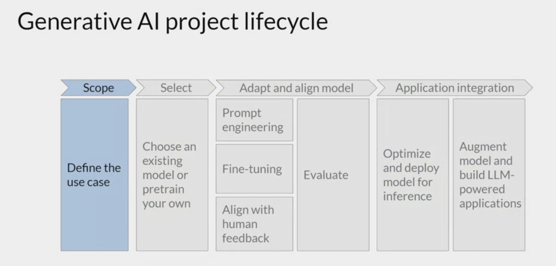
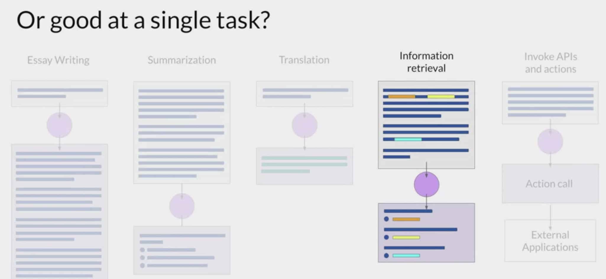
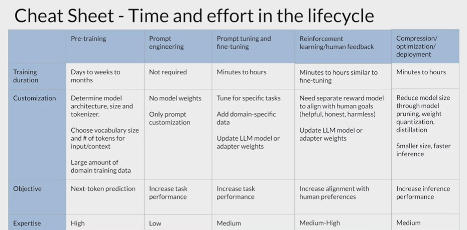
time and effort required for each phase of work.
- pre-training
- pre-training a large language model can be a huge effort.
- themost complex because of the model architecture decisions, the large amount of training data required, and the expertise needed.
- in general will start the development work with an existing foundation model.
- prompt engineering
- start to assess the model’s performance through prompt engineering
- requires less technical expertise, and no additional training of the model.
- prompt tuning and fine tuning
- If the model isn’t performing as you need
- Depending on the use case, performance goals, and compute budget, the methods could range from full fine-tuning to parameter efficient fine tuning techniques like laura or prompt tuning.
- Some level of technical expertise is required for this work.
- fine-tuning can be very successful with a relatively small training dataset
- this phase could potentially be completed in a single day.
- reinforcement learning from human feedback
- Aligning the model using reinforcement learning from human feedback can be done quickly, once you have the train reward model. see if you can use an existing reward model for this work, as you saw in this week’s lab.
- if you have to train a reward model from scratch, it could take a long time because of the effort involved to gather human feedback.
- optimization techniques
- typically fall in the middle in terms of complexity and effort
- can proceed quite quickly assuming the changes to the model don’t impact performance too much.
- After working through all of these steps, trained in tuned a gray LLM that is working well for the specific use case, and is optimized for deployment.
The ability of the model
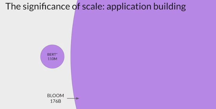
keep in mind as you develop applications using LLMs is the ability of the model to reason well and plan actions depends on its scale.
Larger models are generally the best choice for
techniques that use advanced prompting, like PAL or ReAct.Smaller models may struggle to understand the tasks in highly structured prompts and may requirevadditional fine tuning to improve their ability to reason and plan.
This could slow down the development process.v
start with a large, capable model and collect lots of user data in deployment, use it to train and fine tune a smaller model that you can switch to at a later time.
Interact with external applications
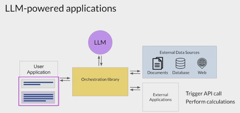
connecting LLMs to external applications allows the model to interact with the broader world, extending the utility beyond language tasks.
LLMs can be used to trigger actions when given the ability to interact with APIs.
- example
- customer service bot
- need to allow the app to process a return requests from end to end.
- customer: want to return some genes that they purchased.
- ShopBot: asking for the order number, which the customer then provides.
- ShopBot: looks up the order number in the transaction database.
- using a RAG implementation
- retrieving data through a SQL query to a back-end order database, no from a corpus of documents.
- ShopBot: retrieved the customers order, confirm the items that will be returned, initiates a request to the company’s shipping partner for a return label.
- uses the shippers Python API to request the label
- customer: email address
- ShopBot: includes this information in the API call to the shipper. let customer know that the label has been sent by email, and the conversation comes to an end.
- LLMs can also connect to other programming resources.
- For example
- Python interpreter that enable models to incorporate accurate calculations into their outputs.
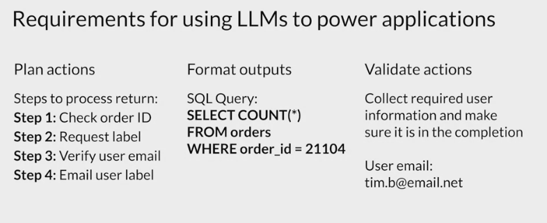
- prompts and completions are at the very heart of these workflows
.
The actions that the app will take in response to user requests will be determined by the LLM, which serves as the application’s reasoning engine.
Structuring the prompts in the correct way is important for all of these tasks and can make a huge difference in the quality of a plan generated or the adherence to a desired output format specification
In order to trigger actions, the completions generated by the LLM must contain certain important information.
- the model needs to be able to generate a set of instructions
so that the application knows what actions to take.
- These instructions need to be understandable and correspond to allowed actions.
- For example: ShopBot checking the order ID, requesting a shipping label, verifying the user email, and emailing the user the label.
- These instructions need to be understandable and correspond to allowed actions.
- the completion needs to be formatted in a way that the broader application can understand .
- a specific sentence structure
- a script in Python or generating a SQL command.
- For example: SQL query that would determine whether an order is present in the database of all orders.
- the model may need to collect information that allows it to validate an action .
ShopBot: verify the email address the customer used to make the original order.
Any information that is required for validation needs to be obtained from the user and contained in the completion so it can be passed through to the application.
- the model needs to be able to generate a set of instructions
LLM application architectures
create end-to-end solutions for the applications
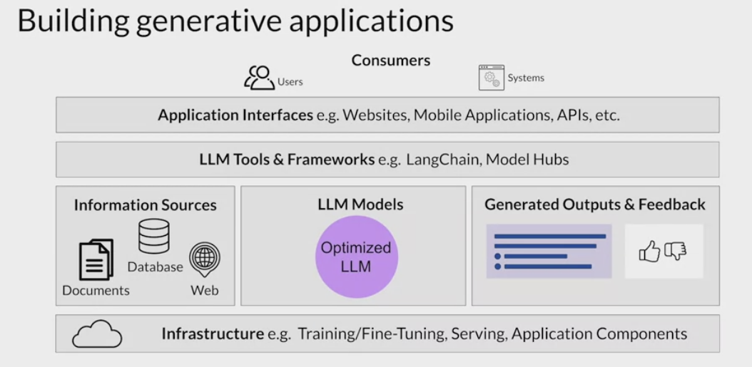
building blocks for creating LLM powered applications.
infrastructure layer.
This layer provides the compute, storage, network to serve up the LLMs and host the application components.
use on-premises infrastructure or on-demand and pay-as-you-go Cloud services.
include the large language models use in the application.
- foundation models
- models you have adapted to the specific task.
The models are deployed on the appropriate infrastructure for the inference needs.
- whether you need real-time or near-real-time interaction with the model.
to retrieve information from external sources (retrieval augmented generation).
return the completions from the large language model to the user or consuming application.
to capture and store the outputs.
to gather feedback from users that may be useful for additional fine-tuning, alignment, or evaluation as the application matures.
use additional tools and frameworks for large language models that help implement some of the techniques
use lengchains built-in libraries to implement techniques like pow react or chain of thought prompting.
utilize model hubs which allow you to centrally manage and share models for use in applications.
user interface that the application will be consumed through, such as a website or a rest API.
- include the security components required for interacting with the application.
Choosing an extraction approach, https://docs.sensible.so/docs/author ↩
Attention is not all you need: pure attention loses rank doubly exponentially with depth, https://arxiv.org/pdf/2103.03404.pdf ↩
The Foundation Model Transparency Index, https://crfm.stanford.edu/fmti/fmti.pdf ↩
LLMSurvey, https://github.com/RUCAIBox/LLMSurvey ↩
Open_LLM_Leaderboard, https://huggingface.co/spaces/HuggingFaceH4/open_llm_leaderboard ↩
Language Models are Unsupervised Multitask Learners, https://d4mucfpksywv.cloudfront.net/better-language-models/language_models_are_unsupervised_multitask_learners.pdf. ↩
Comments powered by Disqus.