Meow's Lab - Riverbed Modeler: Ethernet CSMA/CD & VLAN Lab
Riverbed Modeler: Ethernet CSMA/CD & VLAN Lab
Overview
Two Riverbed Modeler Academic Edition labs covering core LAN performance concepts. Lab 1 studies CSMA/CD Ethernet behavior under varying traffic loads on a 30-node coaxial bus. Lab 2 measures how VLAN segmentation reduces switch broadcast overhead in a multi-building switched Ethernet network for the fictional consulting firm Simple-n-Real.
Both labs use Discrete Event Simulation (DES) to compress hours of real network traffic into minutes of simulation time.
Lab 1: Ethernet CSMA/CD — Direct Link Network with Media Access Control
Objective:
- Demonstrate the operation of an Ethernet network.
- Examine Ethernet performance under different traffic load scenarios.
Background
The Ethernet is a working example of CSMA/CD (Carrier Sense, Multiple Access with Collision Detect) LAN technology.- Multiple access
: all nodes share a common transmission medium.
- Carrier sense
: all nodes can distinguish between an idle and a busy link.
- Collision detect
: a node listens while transmitting; if interference is detected, it stops and retries after a random back-off delay.
- 1-persistent
: an adaptor with a frame to send transmits with probability 1 whenever a busy line goes idle.
The lab sets up an Ethernet with 30 nodes connected via a coaxial link in a bus topology at 10 Mbps.
Step 1 — Create a New Project
**Local area networks (LANs):** designed to span distances of up to a few thousand meters.- Start Riverbed Modeler Academic Edition → File → New.
- Select Project → OK → Name the project:
<initials>_Ethernet, scenario:Coax_2→ check Use Startup Wizard → OK. - In the Startup Wizard: Initial Topology dialog:
- Select Create Empty Scenario → Next
- Network Scale: Office → Next
- X Span: 200, Y Span: 100 → Next → Finish.
- Close the Object Tree dialog box.
Step 2 — Create the Network
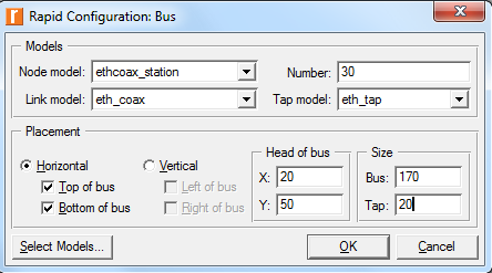
To create the coaxial Ethernet network:- Select Topology → Rapid Configuration → Bus → Next.
- Click Select Models → Model List: **ethcoax** → OK.
- `eth_tap`
: Ethernet bus tap that connects a node to the bus.
- `eth_coax`
: Ethernet bus connecting nodes via taps.
- `eth_tap`
- In the Rapid Configuration dialog, set 30 nodes and click OK.
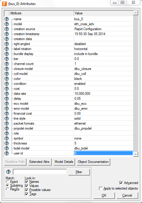
- Right-click the horizontal link → Edit Attributes (Advanced):
- Click model → Edit → select `eth_coax_adv` model.
- Set delay:
0.05(propagation delay in sec/m). - A higher delay is used as an alternative to generating higher traffic, which would require much longer simulation time.
- Set thickness:
5(display width of the bus link). - → OK.
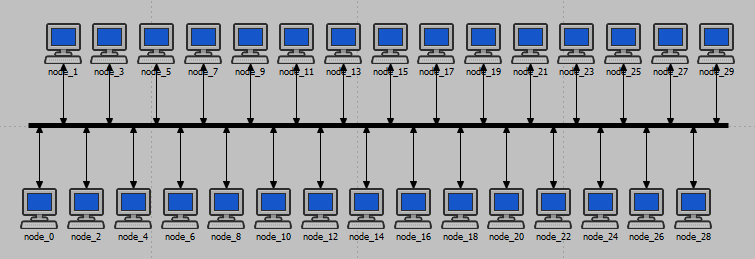
- The network should now look like the illustration below. Save the project.
Step 3 — Configure the Network Nodes
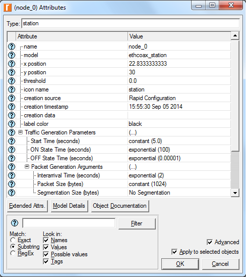
- Right-click any node → Select Similar Nodes (selects all 30).
- Right-click any node → Edit Attributes.
- Check Apply Changes to Selected Objects.
- Expand **Traffic Generation Parameters**:
- ON State Time:
exponential(100) - OFF State Time:
exponential(0.00001) - (Packets are generated only in the ON state.)
- ON State Time:
- Expand **Packet Generation Arguments**:
- Packet Size:
constant(1024) - Interarrival Time:
exponential(2)(mean 2 sec between packets in ON state)
- Packet Size:
- Click OK. Save the project.
Step 4 — Choose Statistics
A probe represents a request by the user to collect a particular piece of data about a simulation.- Right-click workspace (not on a node) → Choose Individual DES Statistics → Expand Global Statistics:
- Traffic Sink
→ check Traffic Received (packets/sec)
- Traffic Source
→ check Traffic Sent (packets/sec)
- Click OK.
- Traffic Sink
- Select DES → Choose Statistics (Advanced):
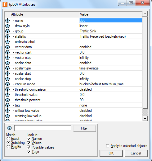
- Right-click Traffic Received probe → Edit Attributes:
- scalar data: enabled
- scalar type: time average
- → OK
- Repeat for the Traffic Sent probe.
- Right-click Traffic Received probe → Edit Attributes:
- Probe Model → File → save → close.
Step 5 — Run Simulation — Multiple Load Scenarios
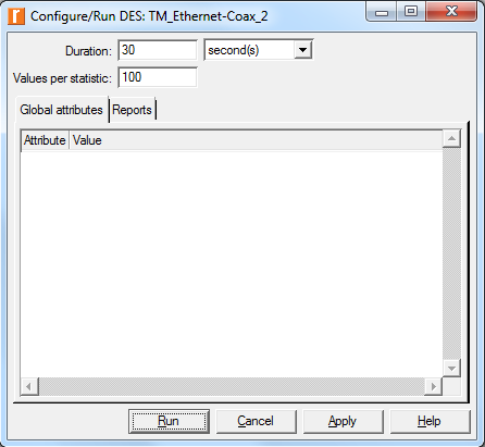
- Click Configure/Run Simulation
 → Duration: 30 seconds → Run.
- After completion, click Close → save project.
- Scenarios → Duplicate Scenario, name
Coax_1. - Repeat duplication, changing Interarrival Time for each scenario:
| Scenario | Interarrival Time | Relative Load |
|---|---|---|
Coax_2 | exponential(2) | Lightest |
Coax_1 | exponential(1) | |
Coax_05 | exponential(0.5) | |
Coax_025 | exponential(0.25) | |
Coax_01 | exponential(0.1) | |
Coax_005 | exponential(0.05) | |
Coax_0035 | exponential(0.035) | |
Coax_003 | exponential(0.03) | |
Coax_0025 | exponential(0.025) | |
Coax_002 | exponential(0.02) | Heaviest |
Step 6 — View Results
- Click View Results
 → open Results Browser.
 - Select the DES Parametric Studies tab.
- From Results for: Current Project, check all results (uncheck
Coax_0025). - Uncheck Include vectors.
- Expand Scalar Statistics → Traffic Sink and Traffic Source.
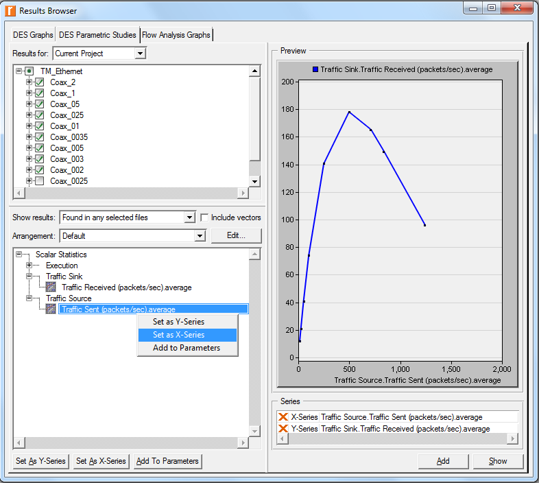
- Right-click Traffic Received → Set as Y-Series.
- Right-click Traffic Sent → Set as X-Series → click Show.
Key observations:
- At very low load
: throughput is near zero — the network is underutilized.
- At medium load
: throughput peaks as traffic saturates the channel efficiently.
- At high load
: collisions multiply, retransmissions waste bandwidth, and throughput collapses.
Lab 1 Discussion Questions
Why does throughput drop at both very low and very high load? At very low load, the channel is mostly idle — few packets arrive so throughput is naturally low. At very high load, every transmission attempt triggers a collision, retransmissions pile up, and useful throughput collapses.
Effect of collision count: Duplicate
Coax_01,Coax_005,Coax_0025. Add Node Statistics → Ethcoax → Collision Count for node 0. Compare collision counts and received traffic across the three scenarios using DES → Results → Compare Results.Effect of station count: Duplicate
Coax_0025asCoax_Q3. Remove the 15 odd-numbered nodes (node 1, 3, … 29). Compare node 0 collision counts betweenCoax_0025andCoax_Q3— fewer nodes reduce collision probability at the same load.Effect of packet size: Duplicate
Coax_0025asCoax_Q4. Change packet size toconstant(512). Compare throughput in packets/sec and bits/sec betweenCoax_0025andCoax_Q4.
Lab 2: Improving LAN Performance Using VLANs
Objective:
- Configure VLANs to improve switch performance.
- Use simulation to make data-driven infrastructure decisions.
Scenario: Simple-n-Real consulting firm — three buildings (A, B, C), each with a switch. User groups: Engineering, Marketing, Sales. Servers provide FTP, Database, HTTP, and email services.
Part 1 — Understand the Baseline Model
- Start Riverbed Modeler Academic Edition → File → Open → LAN_Lab_2.
- Open scenario
Switched_Ethernet_No_VLAN.
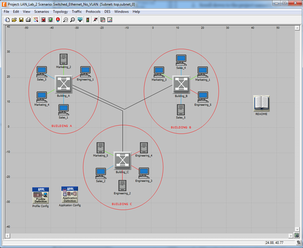
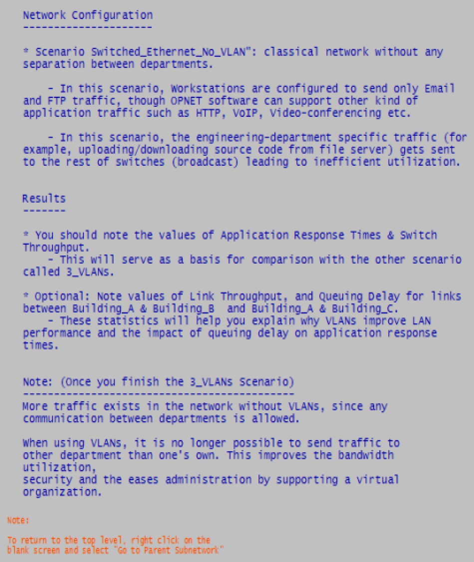
- Read the README file (double-click the
 book icon), then click
  to return to the topology view.
 - Explore Application Config and Profile Config to understand traffic: Email, FTP, HTTP, Database. These values are pre-tuned — changes may alter results significantly.
- Right-click any switch (Building_A, B, or C) → Edit Attributes → expand Switch Port Configuration → expand any port row → expand **VLAN Parameters**:
- Verify Scheme = **Default** — no VLANs configured.
- Click Cancel.
- Right-click the link between Building_A ↔ B or Building_A ↔ C → Edit Attributes → note the link data rate (in bits/sec).
Part 2 — Run the Baseline Simulation
- Click Configure/Run Simulation
 toolbar button.
 - Set Simulation Duration: **8 hours**.
- Click Run — monitor the progress bar.
- When complete, click Close.
Part 3 — View Baseline Results
**View Application Response Times:**- DES → Results → View Results.
- Expand Global Statistics → Email and FTP.
- Select Download Response Time (sec) and Upload Response Time (sec) for both Email and FTP.
- Settings: Stacked Statistics, This Scenario, As Is → click Show.
- Switch As Is dropdown to average → click Add → overlay raw + average curves.
**View Switch Throughput Statistics:**Note: Use the
button in the Results Browser toolbar to toggle individual graph panels on or off.
- Back in View Results, unselect Email/FTP.
- Expand Object Statistics → subnet_0 → Building_A → Switch.
- Select **Traffic Received (bits/sec)** and **Traffic Forwarded (bits/sec)**.
- Settings: Stacked Statistics, This Scenario, As Is → Show → switch to average.
- Repeat for Building_B and Building_C.
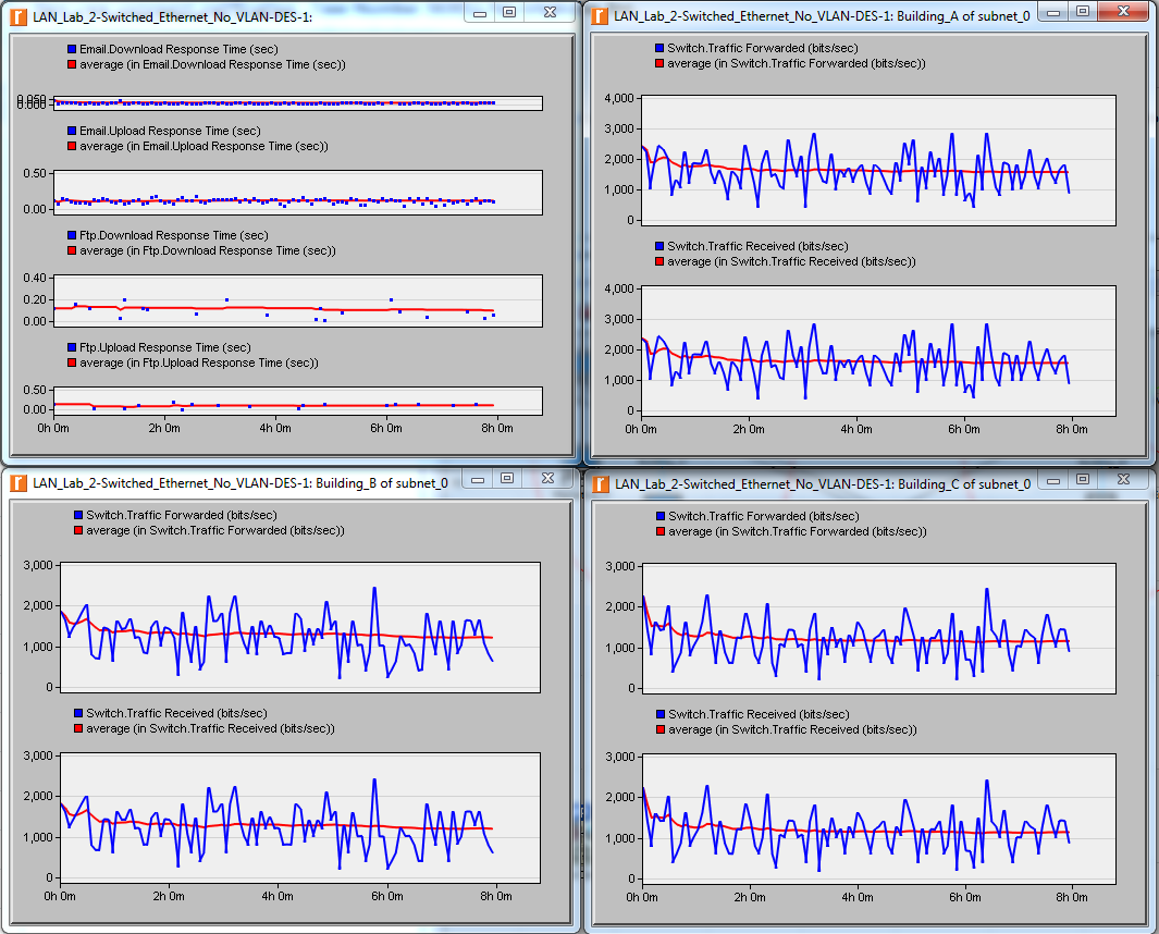
Record baseline values:
| Metric | Min | Max | Avg |
|---|---|---|---|
| Email Download Response Time (sec) | |||
| Email Upload Response Time (sec) | |||
| FTP Download Response Time (sec) | |||
| FTP Upload Response Time (sec) | |||
| Building_A Traffic Received (bits/sec) | |||
| Building_A Traffic Forwarded (bits/sec) | |||
| Building_B Traffic Received (bits/sec) | |||
| Building_B Traffic Forwarded (bits/sec) | |||
| Building_C Traffic Received (bits/sec) | |||
| Building_C Traffic Forwarded (bits/sec) |
Part 4 — Switch to VLAN Scenario and Compare
- Scenarios → Switch Scenarios → choose **3_VLANs**.
- Right-click any switch → Edit Attributes → expand VLAN Parameters:
- Verify Scheme = **Port-Based VLAN** (vs. Default in the previous scenario).
- Click ( … ) next to Supported VLANs → Edit:
- Note the 3 VIDs defined: **10, 20, 30** (one per department: Engineering, Marketing, Sales).
- Click Cancel twice.
- The topology, application, and profiles are identical to the No-VLAN scenario.
- Run the simulation (same 8-hour duration).
- View results following the same steps as Part 3.
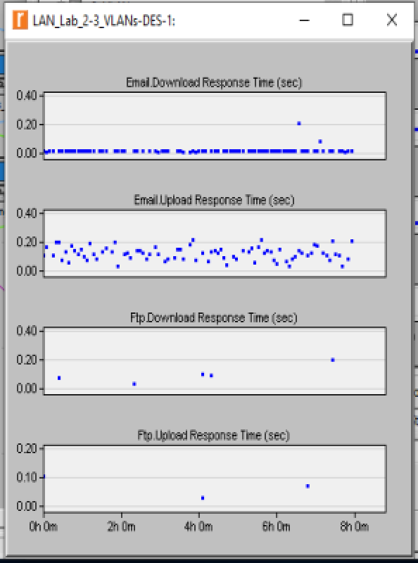
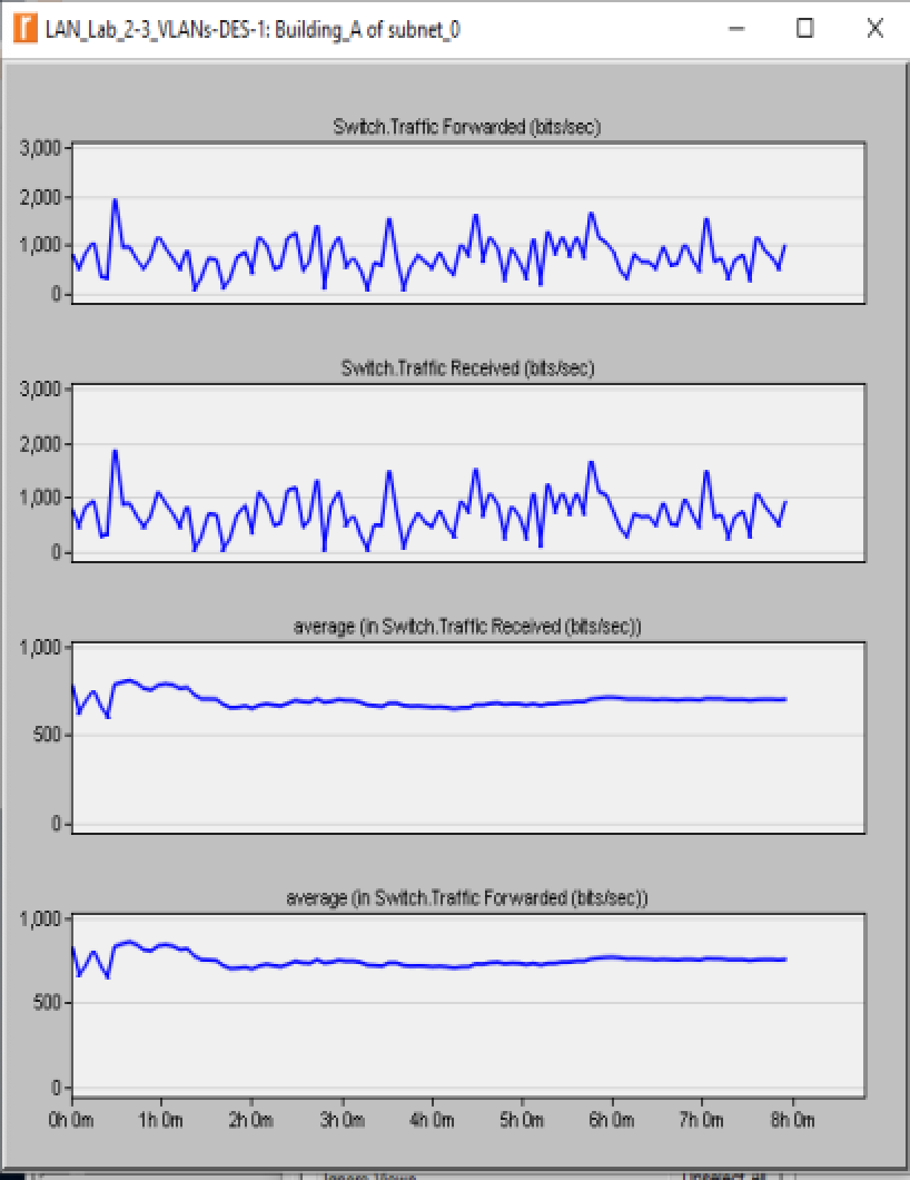
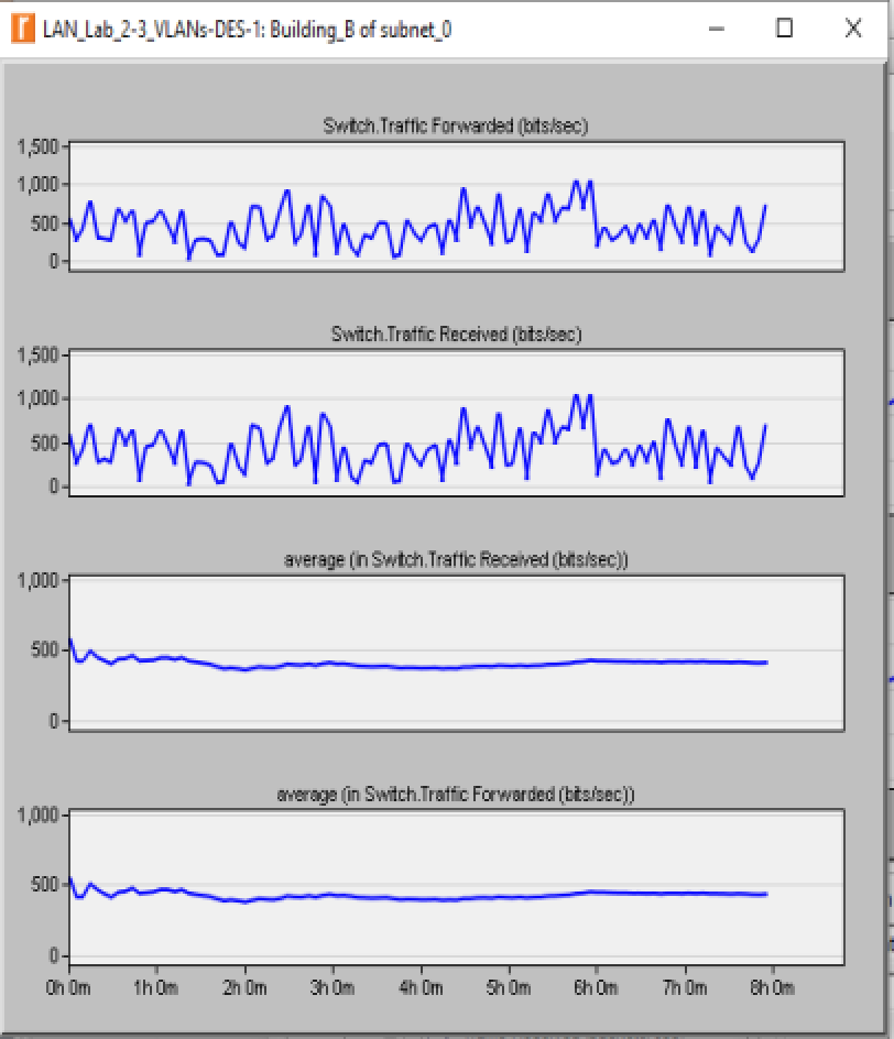
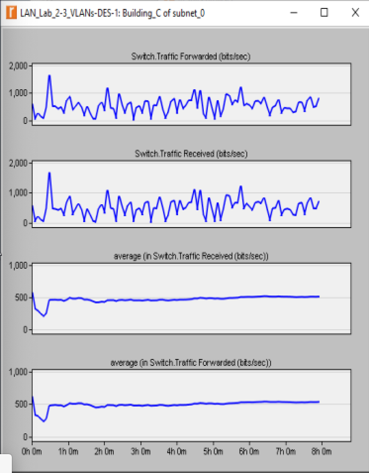
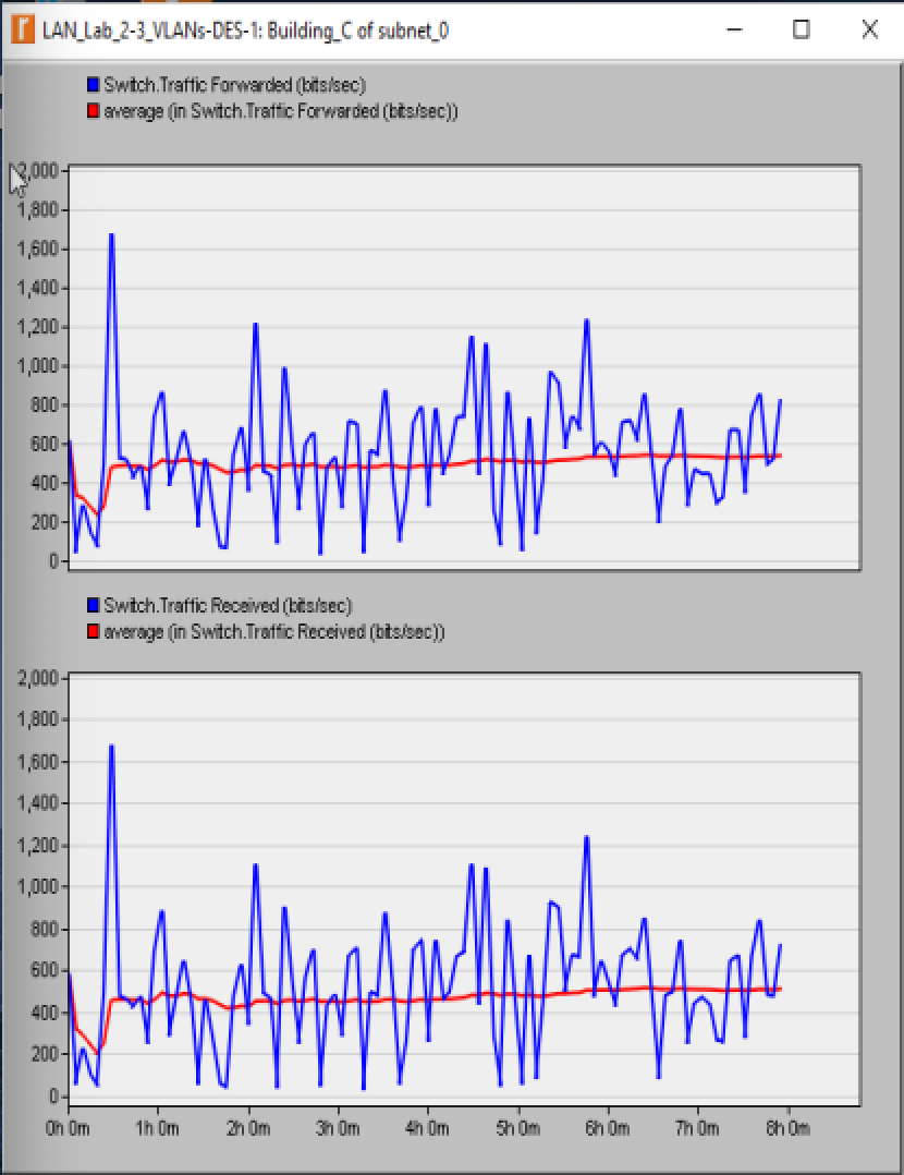
Compare scenarios using DES → Results → Compare Results:
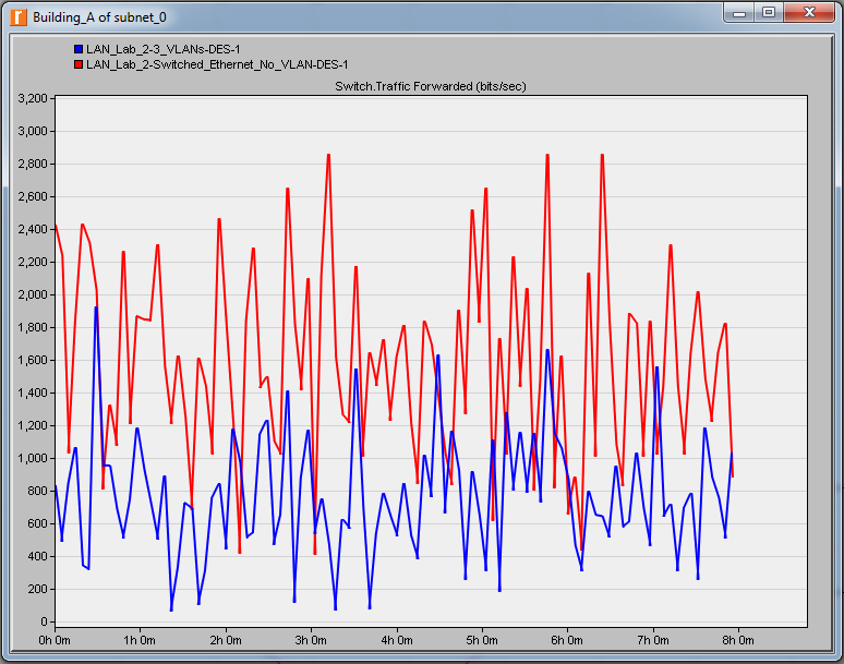
- Select both projects in the top-right pane.
- Plot Object Statistics → subnet_0 → Building_A → Switch → Traffic Forwarded (bits/sec).
- Settings: Overlaid Statistics, average → Show.
Part 5 — Analyze Queuing Delay
Compare queuing delay on the Building_C → Building_A link across both scenarios:
- DES → Results → Compare Results (both projects selected).
- Expand Object Statistics → subnet_0 → Building_A ↔ Building_C → point-to-point.
- Select queuing delay (sec) ←.
- Settings: Overlaid Statistics, average → Show.
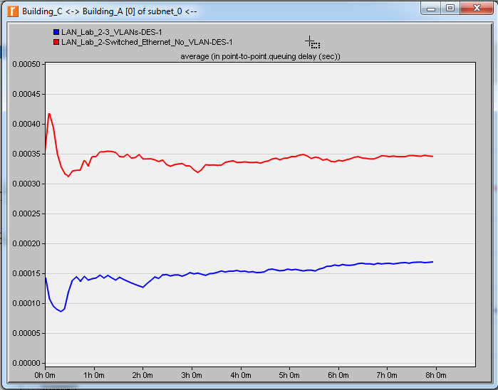
Interpretation:
- Switch throughput drops significantly with VLANs
: broadcast frames are confined within each VLAN — switches no longer flood broadcasts across all three buildings.
- Application response times do not change significantly
: queuing delays are small to begin with, so the reduction is real but too small to materially impact end-to-end response time.
- The amount of application data sent is identical across both scenarios
— only switch forwarding behavior changes.
Key insight: VLAN reduces switch broadcast overhead and improves bandwidth utilization. The benefit to application response time becomes large only when queuing congestion is already significant. VLANs also provide security isolation and administrative flexibility regardless of load.
Network Delay Components:
| Component | Description |
|---|---|
| Bandwidth delay | Time to serialize the packet onto the wire |
| Propagation delay | Speed-of-light travel time across the medium |
| Protocol delay | Processing time in the protocol stack |
| Congestion (queuing) delay | Wait time in switch/router queues — the target metric for VLAN optimization |
Key Takeaways
- CSMA/CD throughput peaks at medium load and collapses at high load
— collisions and retransmissions consume all available bandwidth.
- 1-persistent Ethernet
transmits immediately when the link goes idle — maximizes utilization at low load, maximizes collisions at high load.
- VLAN reduces switch forwarded traffic
by confining broadcast domains — switches no longer flood traffic across the entire network.
- VLAN impact on application response time is small at moderate load
— queuing delays must already be significant for VLAN to materially improve response time.
- VLAN benefits
: bandwidth utilization, security isolation, and administrative flexibility via virtual organization.
- Reducing station count
or packet size reduces collision probability on a shared CSMA/CD medium.
References
- Riverbed Modeler Academic Edition Lab 1: Ethernet CSMA/CD
- Riverbed Modeler Academic Edition Lab 2: Improving LAN Performance Using VLANs
- IEEE 802.1Q — Virtual Bridged Local Area Networks
Comments powered by Disqus.