Meow's 536OS - 11. Mass-Storage Systems

Posted May 25, 2026

By Grace L

21 min read

Mass-Storage Systems

Overview

Secondary storage is the persistent layer beneath main memory — it survives power cycles and holds the bulk of a system’s data. This chapter covers the physical structure of HDD and NVM devices, the scheduling algorithms the OS uses to service I/O requests efficiently, error detection and correction, storage device management (formatting, partitions, boot blocks, bad blocks), swap-space management, how storage is attached to a system (host-attached, NAS, SAN, cloud), and RAID reliability and performance structures.

11.1 Overview of Mass-Storage Structure

11.1.1 HDD Hard Disk Drives

**Disk platter**

: flat circular shape (like a CD). Common diameters: 3.5”, 2.5”, 1.8”. Capacity: 30 GB to 3 TB per drive.

Both surfaces of a platter are coated with magnetic material.
Store information: record magnetically on platters.
Read information: detect the magnetic **pattern** on the platters.

A **read–write head** “flies” just above each platter surface. The heads are attached to a disk arm that moves all heads as a unit.

The surface of a platter is logically divided into:

**Tracks**
: circular rings on the platter surface.
**Sectors**
: subdivisions of tracks; the smallest unit of transfer (historically 512 bytes, now commonly 4 KB).
**Cylinder**
: the set of all tracks at the same arm position across all platters.

Hard Disk Performance

A disk drive motor spins at high speed. Common speeds: 5,400 / 7,200 / 10,000 / 15,000 RPM.

Disk transfer rates:

Rate	Description
Transfer rate (theoretical)	Rate at which bits can be read from media by the disk head (~6 Gb/s)
Effective transfer rate (real)	Rate at which blocks are delivered to the OS (~1 Gb/s)

Transfer rates always > effective transfer rates.

Positioning time / random-access time = seek time + rotational latency:

**Seek time**
: time to move the disk arm to the desired cylinder. Typically 3–12 ms; 9 ms common for desktop drives.
**Rotational latency**
: time for the desired sector to rotate under the disk head. Average latency = ½ full rotation time = 60 / (2 × RPM) seconds.

Key formulas:

\[\text{Access Latency} = \text{Average Seek Time} + \text{Average Rotational Latency}\] \[\text{Average I/O Time} = \text{Access Latency} + \text{Transfer Time} + \text{Controller Overhead}\]

Example — transferring a 4 KB block on a 7200 RPM disk, 5 ms average seek, 1 Gbps transfer rate, 0.1 ms controller overhead:

Transfer time = (4 × 1024 × 8) / 10⁹ ≈ 0.031 ms
Average rotational latency at 7200 RPM = 60 / (2 × 7200) ≈ 4.17 ms
Average I/O time = 5 + 4.17 + 0.031 + 0.1 = 9.301 ms

**head crash**

: if the disk head contacts the disk surface, the magnetic coating is damaged. The entire disk must usually be replaced and data is lost.

HDDs are sealed units. Some chassis allow hot-swap (removal without shutdown). Removable media: CDs, DVDs, Blu-ray.

Drive attached to computer via **I/O bus** — EIDE, ATA, SATA, USB, Fibre Channel, SCSI, SAS, Firewire. A host controller in the computer uses the bus to communicate with the disk controller built into the drive.

11.1.2 NVM Nonvolatile Memory Devices

Nonvolatile memory (NVM)

devices are electrical rather than mechanical.

Composed of a controller and flash NAND die semiconductor chips.
Common forms: SSD (solid-state disk), USB thumb drive, surface-mounted on motherboards.

NVM vs HDD comparison:

Property	NVM (SSD)	HDD
Moving parts	None	Yes
Seek / rotational latency	None	Yes (milliseconds)
Speed	Much faster	Slower
Power consumption	Lower	Higher
Cost per MB	Higher	Lower
Capacity	Smaller (growing fast)	Larger
Lifespan concern	Write wear (DWPD)	Head crash

Because NVM is much faster than HDD, standard bus interfaces can be a bottleneck. **NVMe (NVM Express)** directly connects the NVM device to the system PCIe bus, greatly increasing throughput and reducing latency.

NAND Flash Controller Algorithms

NAND semiconductors cannot be overwritten — data must be erased before a new write:

Read and write occur in page increments (like a sector).
Erase occurs in block increments (multiple pages). Speed: read > write » erase.
Each erase cycle causes write wear. After ~100,000 program-erase cycles, cells no longer retain data.

Lifespan metric: Drive writes per day (DWPD) — how many times the full drive capacity can be written per day within the warranty period.

Controller management techniques:

Technique	Purpose
Flash Translation Layer (FTL)	Maps logical blocks to valid physical pages; tracks which pages/blocks are valid or invalid
Garbage collection	Copies valid pages from partially-invalid blocks; erases all-invalid blocks; reclaims space
Over-provisioning	Sets aside ~20% of capacity as always-available write space; supports GC and wear leveling
Wear leveling	Distributes writes evenly across all blocks so no single block wears out early

write amplification: one application write may trigger additional internal reads, writes, and erases by the GC process, significantly impacting write performance.

11.1.3 Volatile Memory (RAM Drives)

Despite being volatile, DRAM is sometimes used as a mass-storage device via RAM drives:

Device drivers carve out a section of DRAM and present it as a storage device.
File systems can be created on RAM drives for standard file operations.

RAM drives by OS:

Linux: /dev/ram; /tmp is created at boot as tmpfs (a RAM drive).
macOS: diskutil command creates RAM drives.
Windows: via third-party tools.
Solaris/Linux: /tmp as tmpfs.

Magnetic Tapes: early secondary storage. Nonvolatile, large capacity, but random access ~1000× slower than HDD. Used mainly for backup and archival. Sequential access speeds comparable to HDD (≥140 MB/s). Typical storage: 200 GB – 1.5 TB; modern tapes exceed several TB.

11.1.4 Secondary Storage Connection Methods

A secondary storage device is attached to a computer by system bus or I/O bus.

Common bus types:

ATA, SATA, eSATA
— most common for HDDs
Serial Attached SCSI (SAS)
Universal Serial Bus (USB)
Fibre Channel (FC)
**NVMe**
— direct PCIe connection for NVM devices

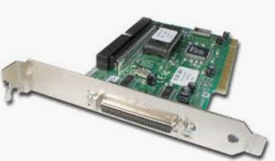
Data transfers on a bus are carried out by controllers (host-bus adapters, HBA):

**Host controller**
: at the computer end of the bus.
**Device controller**
: built into each storage device.

I/O operation flow:

Computer places command into the host controller (via memory-mapped I/O ports).
Host controller sends command to the device controller.
Device controller operates the drive hardware.
Data transfer at the drive: between the device cache and the storage media.
Data transfer to the host: from the device cache to host DRAM via DMA.

11.1.5 Address Mapping

Storage devices are addressed as a large one-dimensional array of **logical blocks**. Each logical block maps to a physical sector (HDD) or semiconductor page (NVM).

HDD mapping: Sector 0 = first sector of the first track on the outermost cylinder. Mapping proceeds through that track, then the rest of the cylinder, then inner cylinders.
NVM mapping: From a tuple (chip, block, page) to an array of logical blocks.

A **Logical Block Address (LBA)** is easier for algorithms to use than a raw physical address tuple.

Why physical-to-logical conversion is non-trivial:

Bad sectors
: controller substitutes spare sectors; LBAs remain sequential but physical locations change.
Number of sectors per track is not constant on some drives.
Manufacturers manage LBA-to-physical mapping internally.

Disk rotation models:

Constant Linear Velocity (CLV)
: bit density uniform; rotation speed increases toward inner tracks. Used in CD-ROM/DVD-ROM.
Constant Angular Velocity (CAV)
: rotation speed constant; bit density decreases from inner to outer tracks. Used in hard disks.

11.2 HDD Scheduling

The OS minimizes access time and maximizes data transfer bandwidth by ordering the I/O request queue.

Access time for platter-based storage = seek time + rotational latency.

Device bandwidth = total bytes transferred / total time from first request to last transfer completion.

When the drive is busy, new requests are placed in a queue of pending requests per device. The OS can reorder this queue to reduce total head movement.

11.2.1 FCFS Scheduling

**First-Come, First-Served (FCFS)**

— also called FIFO.

Simplest algorithm; intrinsically fair but does not provide the fastest service.
Example: queue = 98, 183, 37, 122, 14, 124, 65, 67; head starts at cylinder 53.
- Order: 53 → 98 → 183 → 37 → 122 → 14 → 124 → 65 → 67
- Total head movement: 640 cylinders
- Problem: wild swings (122 → 14) waste time.

11.2.2 SSTF Scheduling

**Shortest Seek Time First (SSTF)**

Selects the request with the minimum seek time from the current head position.
A form of Shortest Job First (SJF) scheduling.
May cause starvation of requests far from the head.
Same example: total head movement = 236 cylinders (much better than FCFS).

11.2.3 SCAN Scheduling (Elevator Algorithm)

**SCAN**

— also called the elevator algorithm.

The disk arm moves from one end of the disk to the other, servicing requests along the way.
At the end, direction is reversed and servicing continues.
Same example: head starts at 53 moving toward 0: 53 → 37 → 14 → 0 → 65 → 67 → 98 → 122 → 124 → 183 → 199.
A new request arriving just behind the head must wait for the arm to reach the end, reverse, and come back.

11.2.4 C-SCAN Scheduling

**Circular SCAN (C-SCAN)**

Variant of SCAN; designed for more uniform wait time.
Moves the head from one end to the other, servicing requests along the way.
When the head reaches the other end, it returns to the beginning without servicing on the return trip.
Treats the disk as circular — the last cylinder wraps to the first.

11.2.5 C-LOOK Scheduling

**C-LOOK**

(version of C-SCAN):

LOOK is a version of SCAN; C-LOOK is a version of C-SCAN.
The arm only goes as far as the last request in each direction, then immediately reverses.
Does not travel all the way to the end of the disk if no requests are there.
More efficient than full SCAN/C-SCAN.

11.2.6 Selection of a Disk-Scheduling Algorithm

Choosing the right scheduler:

Condition	Recommended
Light load / single request	All algorithms behave like FCFS
Heavy load	SCAN / C-SCAN — less starvation
Natural appeal / moderate load	SSTF
Default recommendation	SSTF or LOOK

Linux deadline I/O scheduler:

Maintains separate read and write queues (reads get priority — processes block on reads more than writes).
Queues sorted in LBA order (implementing C-SCAN).
Keeps four queues: two read and two write, one sorted by LBA and one by FCFS.
After each batch, checks FCFS queues for requests older than configured age (default 500 ms); if found, selects that LBA queue next.
RHEL 7 alternatives: NOOP (preferred for NVM/CPU-bound systems) and CFQ (default for SATA drives).

The disk-scheduling algorithm should be written as a separate module of the OS to allow replacement.

11.3 NVM Scheduling

Disk-scheduling algorithms (SSTF, SCAN, etc.) target mechanical HDD head movement minimization. NVM devices have no moving parts, so head movement is irrelevant.

NVM devices commonly use a simple **FCFS** policy.
Linux Noop scheduler: FCFS with merging of adjacent requests.
Some SSD schedulers merge only adjacent write requests (write service time is non-uniform due to NAND properties) while servicing reads in FCFS order.

Performance comparison:

Metric	HDD	NVM/SSD
Sequential read	Good	Good to 10× better
Random I/O (IOPS)	Hundreds	Hundreds of thousands
Write performance	Consistent throughout life	Degrades with wear and fullness

write amplification: one write request can trigger multiple internal reads and writes (garbage collection), severely impacting write performance at high utilization.

11.4 Error Detection and Correction

Error detection and correction is fundamental to memory, networking, and storage.

Technique	Detects	Corrects	Notes
Parity bit	Single-bit errors	No	1 extra bit per byte; XOR-based
Checksum	Multi-bit errors	No	Modular arithmetic on fixed-length words
CRC (Cyclic Redundancy Check)	Multiple-bit errors	No	Hash function; common in networking
ECC (Error-Correcting Code)	Yes	Yes	Uses extra storage; per-sector (HDD) or per-page (NVM)

ECC operation:

When the controller writes a sector/page, it calculates an ECC value and stores it alongside the data.
When the sector/page is read, ECC is recalculated and compared with the stored value.
If they differ → data is corrupted.
- Soft error (few bits): ECC identifies and corrects the bad bits automatically.
- Hard error (too many bits): ECC cannot correct → data is lost.

Error detection and correction are key differentiators between consumer and enterprise products (e.g., ECC DRAM in servers).

11.5 Storage Device Management

11.5.1 Drive Formatting, Partitions, and Volumes

Before a storage device can hold data, it must be initialized through three steps:

Step 1 — Low-level (physical) formatting:

Fills the device with a special data structure for each storage location.
Each sector/page structure: header + data + trailer + ECC.
Most drives are low-level-formatted at the factory.
NVM: pages must be initialized and the FTL created.

Step 2 — Partitioning and volume creation:

Type	Description
Partition	Divides device into groups of blocks/pages; each partition treated as a separate device
Volume	Implicit (a file system placed directly in a partition) or explicit (multiple partitions/devices in a RAID set)

In Linux: fdisk manages partitions; /etc/fstab tells the OS to mount each partition at boot.
Mounting: making a file system available for use.
Linux volume manager lvm2 provides explicit volume management; ZFS integrates volume management and file system.

Step 3 — Logical formatting (creation of a file system):

OS stores initial file-system data structures: free/allocated space maps, initial empty directory.

Raw I/O: some programs bypass the file system and use a partition as a raw block array (no file-system structures). Used for swap space and databases needing direct sector placement. Linux achieves similar access via the DIRECT flag to open().

Cluster: most file systems group blocks into larger clusters.

Device I/O: done in blocks.
File system I/O: done in clusters (more sequential access, fewer random seeks).

11.5.2 Boot Block

For a computer to start, it needs an initial bootstrap loader:

Stored in NVM flash firmware on the motherboard (mapped to a known memory address).
The bootstrap is stored in ROM.
The **Bootstrap loader program** is stored in boot blocks of the boot partition.
Full bootstrap program is stored at a fixed location on the storage device.
Default Linux bootstrap loader: grub2.

Windows boot process:

Firmware runs code in motherboard NVM.
Firmware directs the system to read the MBR (Master Boot Record) from the first logical block of the storage device.
MBR = boot code + partition table (listing partitions and a flag for which to boot from).
System reads the first sector of the boot partition (boot sector), which points to the kernel.
Loads OS subsystems and services.

11.5.3 Bad Blocks

HDDs are prone to failure due to moving parts and tight tolerances.

**Bad blocks**
: one or more sectors become defective.

Handling strategies:

Method	Description
Manual (older IDE disks)	Scan at format time; flag bad blocks as unusable; Linux `badblocks` command for ongoing detection
Sector sparing / forwarding	Controller maintains a bad-block list; low-level formatting sets aside spare sectors; controller remaps bad sector to a spare transparently
Sector slipping	Remaps all sectors from the bad one to the first spare, shifting them down one position to avoid losing the spare’s LBA proximity

Soft error (recoverable): controller spares or slips the block, copies data.
Hard error (non-recoverable): data lost; requires restoration from backup.

NVM bad pages:

Controller maintains a table of bad pages and never marks them as available for writing.
No seek-time loss to worry about — simpler than HDD bad-block management.

11.6 Swap-Space Management

11.6.1 Swap-Space Use

Swap space use varies by OS and memory-management algorithm:

Swapping systems: hold an entire process image (code + data) in swap space.
Paging systems: store pages pushed out of main memory.

Swap space sizing:

Overestimate is better than underestimate (underestimate → system crash).
Solaris: swap = virtual memory exceeding pageable physical memory.
Linux: historically 2× physical RAM; modern algorithms use much less.
Some OS (including Linux) allow multiple swap spaces (files + dedicated partitions) on separate storage devices to spread I/O load.

11.6.2 Swap-Space Location

Swap space can reside in two places:

Location	Description
Normal file system	Large file in the file system; easy to create and resize; managed by normal routines
Raw (dedicated) partition	Separate raw partition with no file-system structure; uses a separate swap-space manager; optimized for speed

Internal fragmentation may increase with raw partitions, but is acceptable because swap data is short-lived (reinitialized at boot).
Adding more swap space to a raw partition requires repartitioning or adding another swap space elsewhere.
Linux supports both approaches; the administrator chooses.

11.7 Storage Attachment

11.7.1 Host-Attached Storage

Host-attached storage

: accessed through local I/O ports.

Includes: HDDs, NVM devices, CD/DVD/Blu-ray, tape drives, SANs.
Most common connection: SATA (one or a few ports on a typical system).
External devices: USB, FireWire, Thunderbolt.
High-end workstations/servers: **Fibre Channel (FC)** — high-speed serial over optical fiber or copper cable; supports multiple hosts and storage devices on a fabric.

11.7.2 Network-Attached Storage (NAS)

**Network-Attached Storage (NAS)**

: provides storage access to other hosts across the network.

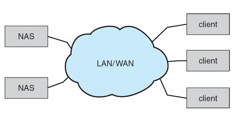
NAS device: special-purpose storage system or a general computer system.
Accessed via **Remote Procedure Calls (RPCs)**:
- **NFS**
  for UNIX/Linux
- **CIFS**
  for Windows
- Both provide file locking for shared access.
RPCs carried via TCP/UDP over IP — usually on the same LAN that carries data traffic.

iSCSI:

Latest NAS protocol.
Carries the SCSI protocol over IP networks instead of SCSI cable.
NFS/CIFS: present a file system, send file parts over the network.
iSCSI: sends logical blocks over the network; client uses blocks directly or creates a file system.

11.7.3 Cloud Storage

**Cloud storage**

: access storage across the Internet/WAN to a remote data center (paid or free).

NAS vs Cloud storage:

	NAS	Cloud Storage
Access protocol	CIFS / NFS / iSCSI (integrated in OS)	Proprietary API (not OS-integrated)
Network	LAN (low latency, reliable)	WAN/Internet (high latency, less reliable)
Failure behavior	NFS/CIFS may hang on LAN failure	Application pauses until connectivity restored

Examples: Amazon S3, Dropbox, Microsoft OneDrive, Apple iCloud.

11.7.4 Storage-Area Networks (SAN) and Storage Arrays

NAS drawback: storage I/O operations consume bandwidth on the general network, increasing latency — especially severe in large client-server installations.

**Storage-Area Network (SAN)**

: a private network using storage protocols (not networking protocols) connecting servers and storage units.

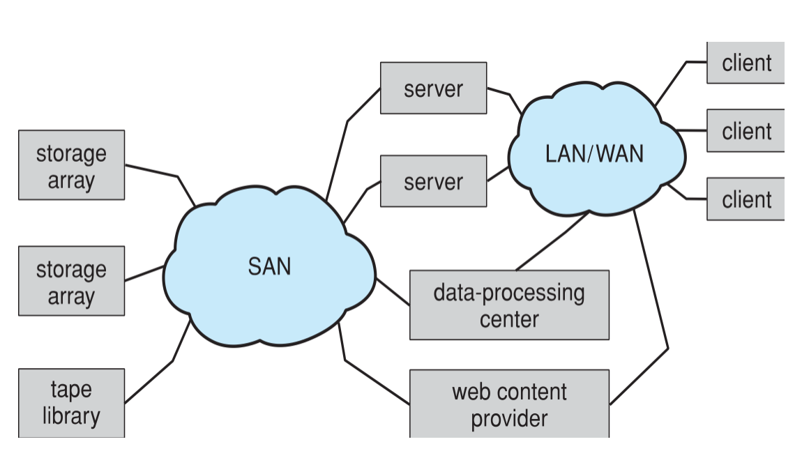
SAN properties:

Property	Description
Flexibility	Multiple hosts and multiple storage arrays on the same SAN
Protocols	FC (most common), iSCSI (growing), InfiniBand (IB)
Storage arrays	RAID-protected arrays or unprotected JBOD (Just a Bunch of Disks)
Dynamic allocation	Storage can be dynamically allocated to hosts as needed
SAN switch	Controls which hosts can access which storage

Storage array: a purpose-built device with SAN/network ports, drives, and a controller (or redundant controllers) composed of CPUs, memory, and software.

Storage array types:

SSD-only: maximum performance, smaller capacity.
Mixed SSD + HDD: SSDs used as cache; HDDs as bulk storage.

SAN vs NAS:

SAN: short distances, no routing, fewer connected hosts possible but dedicated bandwidth.
NAS: can have many more connected hosts; uses general LAN bandwidth.

11.8 RAID Structure

11.8.1 Why RAID?

Storage devices get smaller and cheaper; attaching more drives to a system enables:

Higher transfer rates — drives operated in parallel.
Higher reliability — redundant information stored on multiple drives.

**Redundant Arrays of Independent Disks (RAID)**

: disk-organization techniques addressing performance and reliability. (“I” originally stood for “inexpensive”; now “independent”.)

RAID can be structured as:

Software RAID: OS or system software implements RAID on drives attached to standard buses.
Hardware RAID: intelligent host controller implements RAID on multiple attached devices.
Storage array RAID: standalone unit with its own controller — allows OS without RAID support to use RAID-protected storage.

11.8.2 Improvement of Reliability via Redundancy

With 100 drives each having MTBF = 100,000 hours → MTBF of the array = 100,000 / 100 = 1,000 hours (~41 days). Unacceptable!

Solution: redundancy.

**Mirroring**

(RAID 1):

Duplicate every drive; every write goes to both drives.
A mirrored volume — if one fails, data is read from the other.
MTBF of mirrored volume = MTBF² / (2 × Mean Time to Repair)
- Example: MTBF = 100,000 hr, repair time = 10 hr → 500 × 10⁶ hours ≈ 57,000 years.
Correlated failures (power outage, natural disaster, aging) reduce this theoretical figure.
Write consistency: inconsistent state possible if power fails mid-write. Solutions:
- Write one copy first, then the other.
- Add a solid-state nonvolatile write-back cache (ECC or mirrored) to the RAID array.

11.8.3 Improvement in Performance via Parallelism

Striping data across drives improves transfer rate.

Striping type	Description
Bit-level striping	Bit i of each byte written to drive i; 8 drives act as one drive with 8× access rate
Block-level striping	Block i of a file goes to drive (i mod n) + 1; most commonly used form

Goals of striping parallelism:

Increase throughput of multiple small accesses by load balancing.
Reduce response time of large accesses.

11.8.4 RAID Levels

Level	Name	Technique	Overhead	Read Perf	Write Perf	Fault Tolerance
RAID 0	Block striping	Striping, no redundancy	None	High	High	None
RAID 1	Mirroring	Full duplication	100%	High (can read from either)	Same as single	1 drive failure
RAID 4	Block-interleaved parity	Block striping + dedicated parity drive	1 parity drive	High	Bottleneck at parity drive	1 drive failure
RAID 5	Block-interleaved distributed parity	Parity distributed across all drives	1 drive equivalent	High	Good	1 drive failure
RAID 6	P+Q redundancy	Two independent parity blocks	2 drives equivalent	High	Lower than RAID 5	2 simultaneous failures
RAID 1+0 / 10	Mirror + stripe	Mirrored pairs, then striped	100%	Very high	High	1+ drive failures

RAID 0: block striping without any redundancy. Highest performance but no fault tolerance. Used when performance matters more than reliability (e.g., temporary scratch space).

RAID 1: mirroring. Simple, highly reliable. Write performance same as single drive; read performance up to 2× (both drives can serve reads). Most expensive per usable byte.

RAID 4: dedicated parity drive. Parity computed from corresponding blocks on the data drives (using XOR). Bottleneck: every write must update the parity drive.

RAID 5: distributes parity blocks across all drives — eliminates parity drive bottleneck. Each write updates one data block and one parity block (on different drives). Most popular RAID level.

RAID 6: two independent parity calculations (P+Q) stored across drives. Survives two simultaneous drive failures. Required for large arrays where drive failure during rebuild is a real risk.

RAID 1+0: mirrors drives first (for redundancy), then stripes across pairs (for performance). Combines benefits of RAID 1 and RAID 0.

RAID and NVM: RAID applies to NVM devices too, though NVM devices are less likely to fail than HDDs.

ZFS and Modern Storage Systems

ZFS (originally from Solaris): integrates volume management, RAID (called RAID-Z), and file system into a unified system. Uses end-to-end checksums to detect data corruption in addition to RAID protection.

Key Takeaways

HDD performance is dominated by seek time and rotational latency, not transfer time; minimizing head movement is the primary optimization goal.
NVM/SSD devices eliminate seek and rotational latency but introduce write wear, garbage collection overhead, and write amplification; FCFS (with adjacent-write merging) is the standard scheduling approach.
Disk scheduling algorithms trade fairness (FCFS), locality (SSTF), sweep efficiency (SCAN/C-SCAN), and starvation resistance (LOOK/C-LOOK, Linux deadline scheduler).
ECC is the standard error correction mechanism in both HDDs and NVM devices — soft errors are corrected automatically; hard errors result in lost data.
Swap space can be in a raw partition (faster) or a file-system file (more flexible); Linux supports both.
Storage attachment options span host-attached (SATA, FC), NAS (NFS/CIFS/iSCSI over LAN), cloud (API over WAN), and SAN (dedicated storage fabric with FC or iSCSI).
RAID levels trade redundancy overhead against fault tolerance and performance; RAID 5 is the most common choice; RAID 6 adds protection against double failure; RAID 0 provides performance only.

References

Silberschatz, Galvin, Gagne. Operating System Concepts, 10th Ed. Chapter 11.
Course notes: 536OS chapter 11 Mass-Storage Systems.

00LearningPath, courses

OS mass-storage HDD NVM SSD RAID disk-scheduling FCFS SSTF SCAN C-SCAN C-LOOK NAS SAN swap-space ECC 536OS

This post is licensed under CC BY 4.0 by the author.