Meow's NetworkSec - Ethernet CSMA/CD & VLAN Performance Lab

Ethernet CSMA/CD & VLAN Performance Lab

---

Overview

Two Riverbed Modeler Academic Edition labs covering core LAN concepts. Lab 1 demonstrates CSMA/CD Ethernet bus behavior under varying traffic loads. Lab 2 measures the performance impact of VLAN segmentation on a multi-building switched Ethernet network.

Both labs use Discrete Event Simulation (DES) to observe phenomena that take hours in real networks in minutes of simulation time.

---

Ethernet and CSMA/CD — Concepts

CSMA/CD Protocol

**Carrier Sense, Multiple Access with Collision Detect (CSMA/CD)**

is the MAC protocol underlying classic Ethernet:

• Multiple access

  : all nodes share a common transmission medium

• Carrier sense

  : all nodes can distinguish between an idle and a busy link — a node waits until the link is idle before transmitting

• Collision detect

  : a node listens while transmitting; if it detects interference (a collision), it stops and retries after a random back-off delay

• 1-persistent

  : when the link becomes idle, a node with a frame ready transmits immediately (probability 1)

Ethernet is said to be 1-persistent because an adaptor with a frame to send transmits with probability 1 whenever a busy line goes idle. This maximizes throughput at low load but causes more collisions at high load.

Throughput vs. Load Behavior

Under low load, most transmissions succeed without collision and throughput is close to the offered load. As load increases past a saturation point, collisions multiply, retransmissions consume bandwidth, and effective throughput drops. At very high load, nearly all transmission attempts collide and throughput collapses.

Network Delay Components

Components of network delay on a LAN:

Component	Description
Bandwidth delay	Time to serialize the packet onto the wire
Propagation delay	Speed-of-light travel time across the medium
Protocol delay	Processing time in the protocol stack
Congestion (queuing) delay	Wait time in switch/router queues when links are saturated

On a lightly loaded LAN, bandwidth and propagation delays dominate. Queuing delay only becomes significant when switch queues fill up under heavy traffic.

---

Lab 1: Ethernet Bus Simulation

Objective: Demonstrate CSMA/CD Ethernet operation and measure network throughput under different traffic loads using a 30-node coaxial bus at 10 Mbps.

Create a New Project

**Local area networks (LANs):** designed to span distances of up to a few thousand meters.

1. Start Riverbed Modeler Academic Edition → File → New
2. Select Project → OK → Name the project: <initials>_Ethernet, scenario: Coax_2
3. Check **Use Startup Wizard** → OK
4. In the Startup Wizard: Initial Topology dialog:
   • Select **Create Empty Scenario** → Next
   • Network Scale: Office → Next
   • X Span: 200, Y Span: 100 → Next → Finish
5. Close the Object Tree dialog box

Create the Network

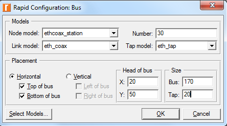
To create the coaxial Ethernet network:

1. Select Topology → Rapid Configuration → Bus → Next
2. Click Select Models → Model List: **ethcoax** → OK
   • `eth_tap`

     : Ethernet bus tap that connects a node to the bus

   • `eth_coax`

     : Ethernet bus connecting nodes via taps

3. In the Rapid Configuration dialog, set 30 nodes and click OK

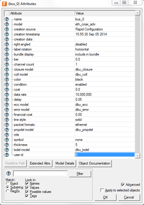
1. Right-click the horizontal link → Edit Attributes (Advanced):
   • Click model → Edit → select `eth_coax_adv` model
   • Set delay: 0.05 (propagation delay in sec/m)
   • A higher delay is used as an alternative to generating higher traffic, which would require much longer simulation time.
   • Set thickness: 5 (display width of the bus link)
   • → OK

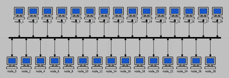
Configure Network Nodes

1. Right-click any node → Select Similar Nodes (selects all 30)
2. Right-click any node → Edit Attributes
3. Check Apply Changes to Selected Objects
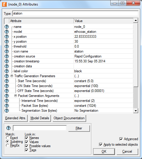
4. Expand **Traffic Generation Parameters**:
   • **ON State Time**

     : exponential(100)

   • **OFF State Time**

     : exponential(0.00001)

   • (Packets are generated only in the ON state)
5. Expand **Packet Generation Arguments**:
   • **Packet Size**

     : constant(1024)

   • **Interarrival Time**

     : exponential(2) (mean 2 sec between packets in ON state)

The exponential distribution argument is the mean interval between successive events. Packet inter-arrival time determines the traffic intensity injected into the network.

Choose Statistics

1. Right-click workspace (not on a node) → Choose Individual DES Statistics
2. Expand Global Statistics:
   • Traffic Sink

     → check Traffic Received (packets/sec)

   • Traffic Source

     → check Traffic Sent (packets/sec)

3. Select DES → Choose Statistics (Advanced):
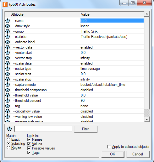
   • Right-click Traffic Received probe → Edit Attributes:
     • scalar data: enabled
     • scalar type: time average
   • Repeat for Traffic Sent probe
4. Probe Model → File → save → close

Run Simulation — Multiple Load Scenarios

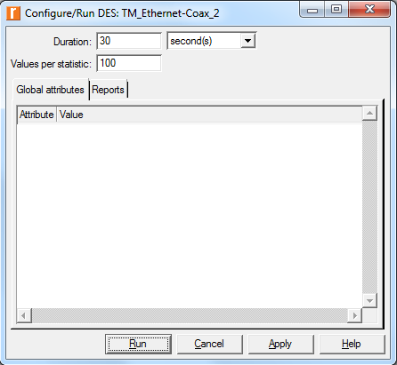
1. Click Configure/Run Simulation → Duration: 30 seconds → Run

1. After completion, click Close → save project
2. Scenarios → Duplicate Scenario, name Coax_1
3. Repeat duplication, changing Interarrival Time for each scenario:

Scenario	Interarrival Time	Relative Load
Coax_2	exponential(2)	Lightest
Coax_1	exponential(1)
Coax_05	exponential(0.5)
Coax_025	exponential(0.25)
Coax_01	exponential(0.1)
Coax_005	exponential(0.05)
Coax_0035	exponential(0.035)
Coax_003	exponential(0.03)
Coax_0025	exponential(0.025)
Coax_002	exponential(0.02)	Heaviest

Each successive run takes longer to complete because traffic intensity is increasing — the network is experiencing more collisions and retransmissions.

View Results

1. Click View Results → open Results Browser
2. Select the DES Parametric Studies tab
3. From Results for: Current Project, check all results (uncheck Coax_0025)
4. Uncheck Include vectors
5. Expand Scalar Statistics → Traffic Sink and Traffic Source
6. Right-click Traffic Received → Set as Y-Series
7. Right-click Traffic Sent → Set as X-Series → click Show

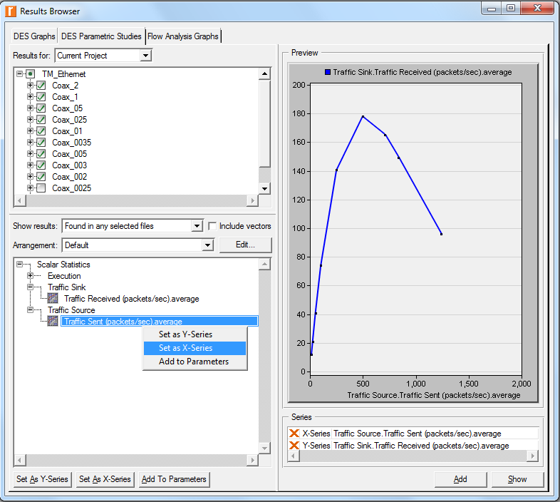
Key observations:

• At low load

  : throughput is near zero because few packets are sent — the network is underutilized

• At medium load

  : throughput peaks as traffic saturates the channel efficiently

• At high load

  : collisions multiply, retransmissions waste bandwidth, and throughput collapses below the peak

Lab 1 Discussion Questions

1. Why does throughput drop at both very low and very high load?
   • At very low load, the channel is mostly idle — few packets arrive, so throughput is naturally low. At very high load, every transmission attempt triggers a collision, retransmissions pile up, and useful throughput collapses.

2. Effect of collision count: As interarrival time decreases (higher load), collision count at any node increases. Comparing Coax_01, Coax_005, Coax_0025 shows the collision count rising while received traffic falls past saturation.

3. Effect of station count: Removing half the nodes (e.g., Coax_Q3 with 15 nodes vs. Coax_0025 with 30) reduces collision probability — fewer nodes contend for the shared medium at the same instant.

4. Effect of packet size: Larger packets hold the medium longer, increasing collision probability at high load. Comparing 1024-byte vs. 512-byte packets (Coax_Q4) shows that smaller packets improve throughput per unit time at heavy load.

---

VLAN — Concepts and Benefits

What is a VLAN?

A Virtual LAN (VLAN) is a logical grouping of network devices into separate broadcast domains, regardless of their physical location. Without VLANs, every frame sent to the broadcast address (FF:FF:FF:FF:FF:FF) is flooded to every port on every switch in the network. In a large flat network, this broadcast traffic consumes significant switch bandwidth and CPU cycles on every device.

VLAN benefits:

Benefit	Description
Bandwidth efficiency	Broadcast traffic is confined within each VLAN — switches do not forward broadcasts across VLAN boundaries
Security	Devices in different VLANs cannot communicate directly — inter-VLAN traffic must pass through a router or Layer 3 switch with access control
Administration	Virtual organization mirrors the logical org chart rather than physical wiring — moves and changes require software config, not cable changes

Port-Based vs. Tagged VLANs

• **Port-Based VLAN**

  : each switch port is statically assigned to one VLAN. Simple and deterministic.

• **802.1Q Tagged VLAN (Trunk)**

  : frames carry a VLAN ID (VID) tag in the Ethernet header, allowing a single trunk link to carry multiple VLANs between switches.

---

Lab 2: VLAN Performance Improvement

Objective: Measure how VLAN segmentation reduces switch broadcast overhead and improves bandwidth utilization in a multi-building switched Ethernet network.

Scenario: Simple-n-Real consulting firm — three buildings (A, B, C), each with a switch. User groups: Engineering, Marketing, Sales. Servers provide FTP, Database, HTTP, and email services.

Part 1: Understand the Baseline (No VLAN)

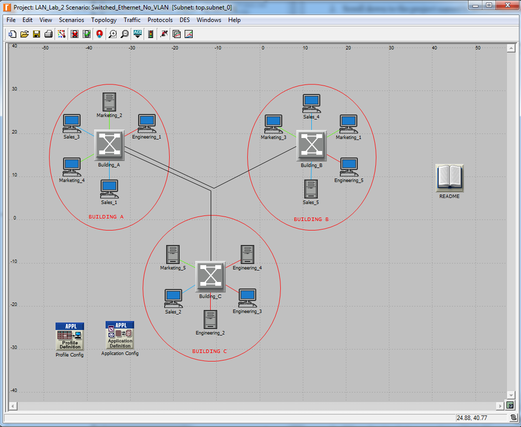
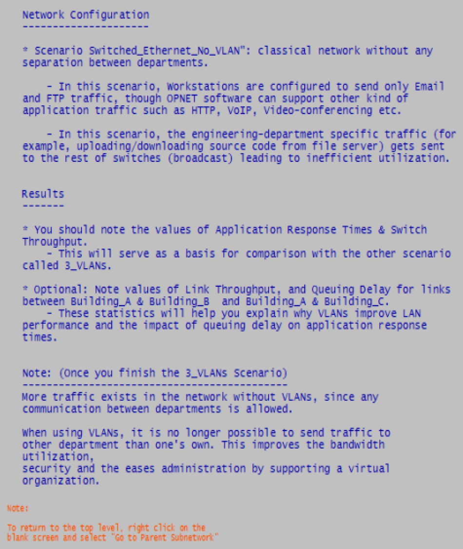
1. Open scenario LAN_Lab_2 → Switched_Ethernet_No_VLAN
2. Read the README file (double-click the book icon), then click to return to the topology view
3. Examine Application Config and Profile Config to understand traffic: Email, FTP, HTTP, Database
4. Right-click any switch (Building_A, B, or C) → Edit Attributes
5. Expand Switch Port Configuration → expand any port row → expand **VLAN Parameters**
   • Verify Scheme = **Default** — this confirms no VLANs are configured
6. Right-click the link between Building_A ↔ B or Building_A ↔ C → Edit Attributes → note the link data rate

Part 2: Run the Simulation

1. Click Configure/Run Simulation toolbar button
2. Set Simulation Duration: **8 hours**
3. Click Run — monitor the progress bar
4. When complete, click Close

Part 3: View Results — Baseline (No VLAN)

**View Application Response Times:**

1. DES → Results → View Results
2. Expand Global Statistics → Email and FTP
3. Select Download Response Time (sec) and Upload Response Time (sec) for both Email and FTP
4. Settings: Stacked Statistics, This Scenario, As Is → click Show
5. Switch As Is dropdown to average → click Add → overlay raw + average curves

Note: Use the button in the Results Browser toolbar to toggle individual graph panels on or off.

**View Switch Throughput Statistics:**

1. Back in View Results, unselect Email/FTP
2. Expand Object Statistics → subnet_0 → Building_A → Switch
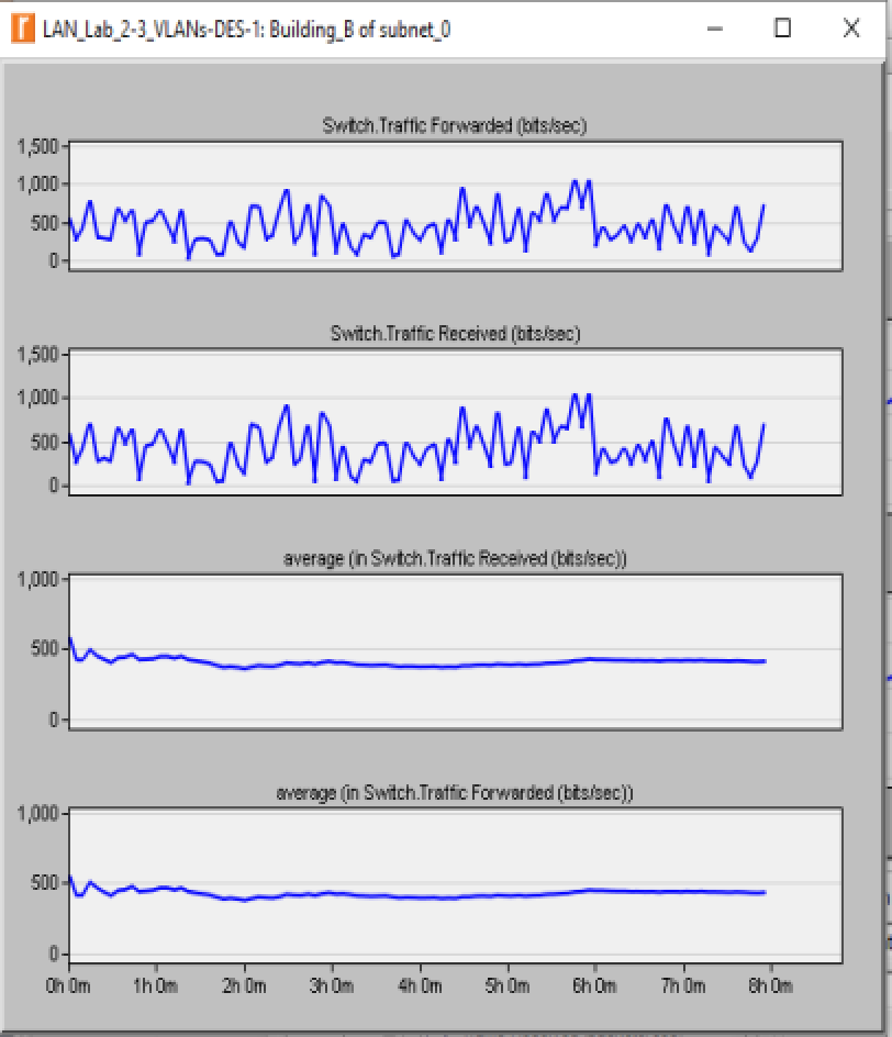
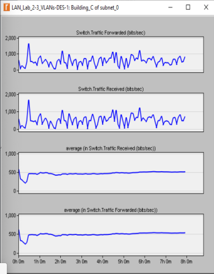
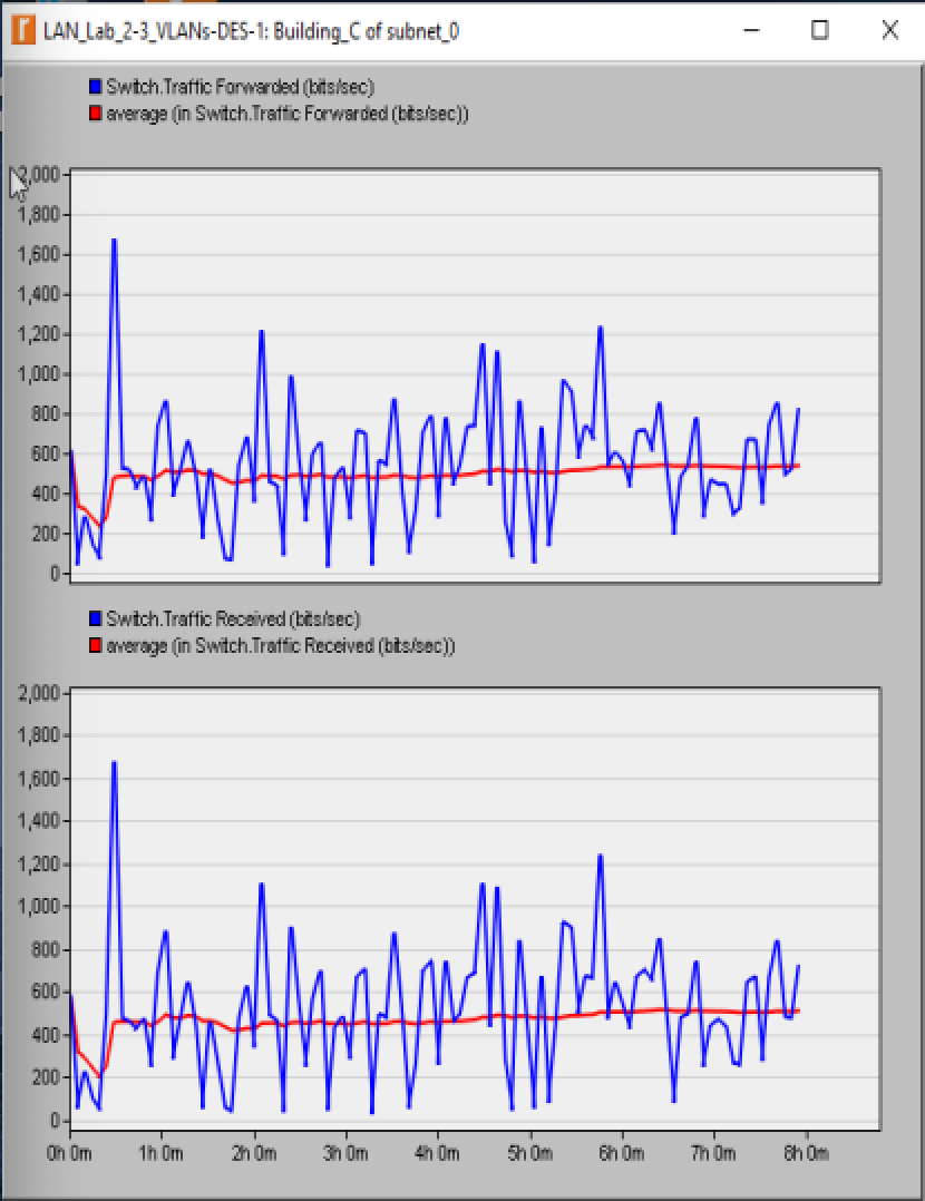
3. Select **Traffic Received (bits/sec)** and **Traffic Forwarded (bits/sec)**
4. Settings: Stacked Statistics, This Scenario, As Is → Show → switch to average
5. Repeat for Building_B and Building_C

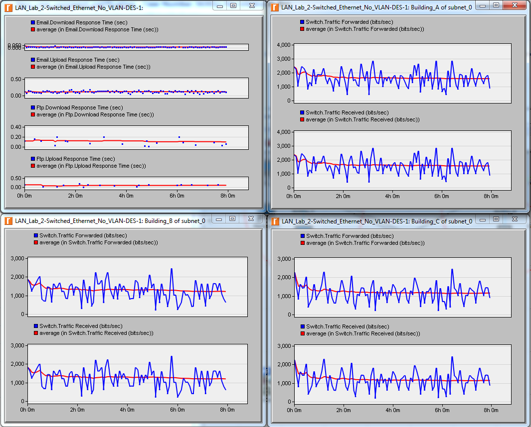
Record baseline values:

Metric	Min	Max	Avg
Email Download Response Time (sec)
Email Upload Response Time (sec)
FTP Download Response Time (sec)
FTP Upload Response Time (sec)
Building_A Traffic Received (bits/sec)
Building_A Traffic Forwarded (bits/sec)
Building_B/C Traffic Received/Forwarded

Part 4: Switch to VLAN Scenario and Compare

1. Scenarios → Switch Scenarios → choose **3_VLANs**
2. Right-click any switch → Edit Attributes → expand VLAN Parameters
   • Verify Scheme = **Port-Based VLAN** (vs. Default in the previous scenario)
3. Click ( … ) next to Supported VLANs → Edit
   • Note the 3 VIDs defined: **10, 20, 30** (one per department: Engineering, Marketing, Sales)
4. Run the simulation (same 8-hour duration)
5. View results following the same steps as Part 3

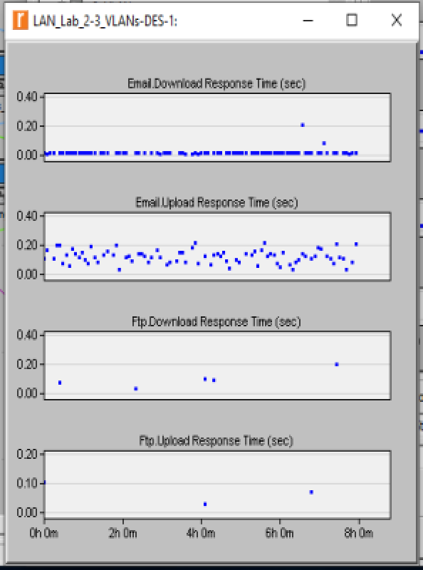
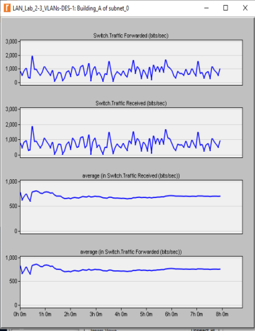
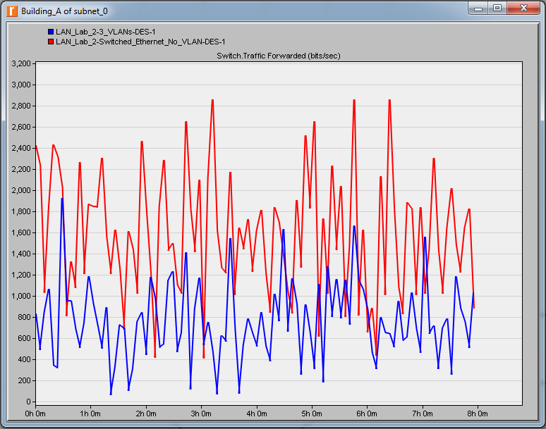
Compare scenarios using DES → Results → Compare Results:

• Select both projects in the top-right pane
• Plot Object Statistics → subnet_0 → Building_A → Switch → Traffic Forwarded (bits/sec)
• Settings: Overlaid Statistics, average

Analysis: VLAN Impact on Queuing Delay

Compare the queuing delay on the link between Building_C and Building_A across both scenarios:

1. DES → Results → Compare Results (both projects selected)
2. Expand Object Statistics → subnet_0 → Building_A ↔ Building_C → point-to-point
3. Select queuing delay (sec) ←
4. Settings: Overlaid Statistics, average → Show

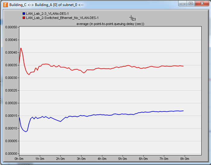
Key observations:

• Switch throughput drops significantly with VLANs

  : broadcast frames are no longer flooded across all three buildings — each VLAN contains its own broadcast domain within its department.

• Application response times do not change significantly

  : queuing delays are very small to begin with (queues are not filled up enough to cause packet dropping). The reduction in queuing delay from VLANs is real but too small to materially impact end-to-end response time.

• The amount of application data sent by workstations is identical across both scenarios

  — the topology, application, and profile configurations are unchanged. Only the switch forwarding behavior changes.

Key insight: VLAN configuration reduces switch broadcast overhead and improves bandwidth utilization. The benefit to application response times becomes large only when queuing congestion is already significant (heavily loaded network). VLANs also provide security and administrative benefits regardless of the load level.

---

Meow’s Security Considerations 安全注意事项

VLAN配置能减少广播域、改善性能，但同时也引入了与VLAN隔离机制相关的安全风险。以下涵盖VLAN跳跃攻击、中继端口误配、CAM表溢出等核心威胁。

VLAN segmentation improves performance and provides logical isolation, but the isolation is enforced in software and can be bypassed through several well-documented attack techniques.

Severity 严重程度	Concern 问题
Critical 严重	VLAN Hopping via switch spoofing — attacker trunk-negotiates into all VLANs
High 高	Double-tagging VLAN hopping — crafted 802.1Q frames reach foreign VLANs
High 高	CAM table flooding — switches degrade to hub behavior, broadcasting all frames
Medium 中	Default VLAN 1 carries management traffic alongside user traffic
Low 低	VLAN misconfiguration exposes cross-department traffic paths

---

1. VLAN Hopping — Switch Spoofing 交换机欺骗 — Critical

攻击者将自己的设备配置为支持DTP（动态中继协议）的交换机，诱使目标交换机与其建立中继链路（trunk link）。一旦中继建立，攻击者可以访问所有VLAN的流量，完全绕过VLAN隔离。

An attacker configures their device to negotiate a trunk link using DTP (Dynamic Trunking Protocol). Once the trunk is established, the attacker’s device receives frames from all VLANs, bypassing segmentation entirely.

攻击向量 Attack Vectors:

• 攻击者连接到一个端口，发送DTP帧，诱使交换机切换为trunk模式 / Attacker connects to an access port and sends DTP frames to trick the switch into trunk mode
• 攻击者随后注入任意VLAN ID的帧，访问任意网段 / Attacker then sends frames tagged with any VLAN ID, accessing any segment

缓解措施 Mitigation: 在所有用户端口上禁用DTP并强制设置为access模式（switchport mode access + switchport nonegotiate）。只在确实需要传输多VLAN流量的上行链路上配置trunk口。 Disable DTP on all user-facing ports (switchport mode access + switchport nonegotiate). Configure trunk mode only on uplinks that genuinely carry inter-switch traffic.

---

2. Double-Tagging VLAN Hopping 双层标签跳跃 — High

攻击者构造一个携带双重802.1Q标签的帧：外层标签是本征VLAN（native VLAN），内层标签是目标VLAN。当第一台交换机剥除外层标签后，内层标签成为有效标签，帧被转发到目标VLAN。

An attacker crafts a frame with two nested 802.1Q tags. The outer tag matches the native VLAN; the inner tag specifies the target VLAN. The first switch strips the outer tag and forwards the frame — now tagged only with the inner (target) VLAN ID — into the victim network segment.

攻击向量 Attack Vectors:

• 攻击者发送双标签帧 → 第一台交换机剥除外层标签 → 第二台交换机转发至目标VLAN / Attacker sends double-tagged frame → first switch strips outer tag → second switch forwards to target VLAN
• 此攻击为单向攻击，无法直接收到目标VLAN的响应 / This is a one-way attack — responses cannot be routed back without additional compromise

缓解措施 Mitigation: 将native VLAN修改为一个未分配给任何用户的专用VLAN ID（例如VLAN 999），并在trunk口上明确禁用该native VLAN的流量传输。 Change the native VLAN to a dedicated, unused VLAN ID (e.g., VLAN 999) and explicitly prune native VLAN traffic from all trunk ports.

---

3. CAM Table Flooding — MAC Flooding MAC地址表溢出 — High

攻击者向交换机发送大量伪造源MAC地址的帧，将交换机的CAM表（内容可寻址内存表）填满。当CAM表溢出时，交换机无法查找目标MAC地址，退化为集线器行为，将所有帧广播到所有端口（包括所有VLAN的端口，如果跨VLAN flooding未被限制）。

An attacker floods the switch with frames carrying random source MAC addresses, exhausting the CAM table. Once full, the switch cannot make forwarding decisions and broadcasts all frames to all ports — allowing the attacker to intercept traffic from any VLAN reachable on that switch.

攻击向量 Attack Vectors:

• 使用macof等工具快速生成随机MAC地址帧，耗尽CAM表 / Tools like macof generate thousands of random MAC frames per second to exhaust the table
• 交换机退化为hub，攻击者可嗅探同一交换机上其他VLAN的所有流量 / Switch degrades to hub — attacker sniffs all traffic on the switch, across VLANs

缓解措施 Mitigation: 启用端口安全（Port Security），限制每个端口可学习的MAC地址数量，超过阈值后关闭端口或丢弃帧。 Enable Port Security to limit the number of MAC addresses learned per port; shut down or restrict the port when the threshold is exceeded.

---

4. Default VLAN 1 Management Exposure 默认VLAN 1暴露 — Medium

VLAN 1是大多数交换机的默认VLAN，通常承载STP（生成树协议）、CDP（Cisco发现协议）、VTP（VLAN中继协议）等管理协议流量。若用户数据和管理流量共享VLAN 1，攻击者可以嗅探管理帧或注入伪造的协议报文。

VLAN 1 is the default VLAN on most switches and carries management protocol traffic (STP, CDP, VTP). If user data shares VLAN 1, attackers can sniff management frames or inject crafted protocol packets.

缓解措施 Mitigation: 将管理流量迁移到专用的管理VLAN，VLAN 1仅保留为从不分配用户的空VLAN。 Move all management traffic to a dedicated management VLAN. Leave VLAN 1 as an empty, never-assigned VLAN.

---

Summary Table 汇总表

#	问题 Concern	MITRE / CWE	状态 Status
1	VLAN Hopping — Switch Spoofing	MITRE T1599 / CWE-284	Mitigate: disable DTP
2	Double-Tagging VLAN Hopping	MITRE T1599.001 / CWE-284	Mitigate: change native VLAN
3	CAM Table Flooding	MITRE T1040 / CWE-400	Mitigate: Port Security
4	Default VLAN 1 Management Exposure	CWE-16	Mitigate: dedicated mgmt VLAN

---

Key Takeaways

• CSMA/CD throughput peaks at medium load and collapses at high load

  — collisions and retransmissions consume all available bandwidth

• 1-persistent Ethernet

  : transmits immediately when the link goes idle — maximizes utilization at low load, maximizes collisions at high load

• VLAN reduces switch throughput

  by confining broadcast domains — fewer frames are flooded across the network

• VLAN impact on application response time is small at moderate load

  because queuing delays are already negligible — the benefit grows under congested conditions

• VLAN benefits

  : bandwidth utilization, security isolation, and administrative flexibility via virtual organization

• VLAN hopping

  (switch spoofing, double-tagging) and CAM flooding are the primary Layer 2 attacks against VLANs — mitigated by disabling DTP, changing the native VLAN, and enabling Port Security

• Network delay components

  : Bandwidth, Propagation, Protocol, Congestion (Queuing) — queuing delay is the target metric for VLAN optimization

References

• Riverbed Modeler Academic Edition lab materials
• IEEE 802.1Q — Virtual Bridged Local Area Networks
• MITRE ATT&CK T1599 — Network Boundary Bridging