Meow's 528CN - 1.5 Network Performance: Bandwidth, Latency & Delay×Bandwidth
1.5 Network Performance: Bandwidth, Latency & Delay×Bandwidth
Source: CS 528 Computer Networks — Chapter 1: Foundation
Overview
Network performance is a first-class design constraint. The effectiveness of computations distributed over a network often depends directly on the efficiency with which the network delivers data. While the programming adage “first get it right, then make it fast” applies in many settings, in networking it is usually necessary to design for performance from the start. This note covers the fundamental metrics — bandwidth, latency, and the delay×bandwidth product — and their implications for high-speed networks, application design, and hardware bottleneck analysis.
1. Bandwidth and Latency 带宽与延迟
Network performance is measured in two fundamental ways: bandwidth and latency.
1.1 Bandwidth 带宽
Bandwidth(throughput) has two related meanings:
- In Hz: the width of a frequency band a medium can carry.
- Example: a voice-grade telephone line supports 300–3300 Hz → bandwidth = 3000 Hz.
- Required bit rate:
8 bits × 3×10³ Hz = 24 Kbps
- In bps (network context): the number of bits that can be transmitted over the network per unit time — the data rate.
Thinking about bandwidth as bit width:
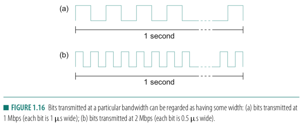
On a 10 Mbps network (10,000,000 bits/sec), each bit occupies 1/10,000,000 = 0.1 μs of transmission time. Intuitively: if time is a ruler and bandwidth is how many bits fit per unit length, then each bit is a pulse of some width — higher bandwidth means narrower bits.
- 1 Mbps link → each bit is 1 μs wide
- 2 Mbps link → each bit is 0.5 μs wide
The more sophisticated the transmitter/receiver technology, the narrower each bit can become, and thus the higher the bandwidth.
A useful distinction exists between:
- Maximum available data rate
on the physical link
- Actual achievable throughput
over a logical process-to-process channel (influenced by software handling, protocol overhead, and data transformations at each hop)
1.2 Latency 延迟
Latency(delay): how long it takes a message to travel from one end of a network to the other.
- One-way latency
: time for a message to travel from source to destination (e.g., 24 ms)
- Round-Trip Time (RTT)
: time to send a message and receive a response — more operationally important than one-way latency
Three components of latency:
| Component | Description |
|---|---|
| Propagation delay | Speed-of-light travel time across the medium |
| Transmission delay | Time to put all bits of a packet onto the wire = packet size / bandwidth |
| Queuing delay | Wait time in switch/router queues before a packet is forwarded on an outbound link |
Propagation speed across media:
| Medium | Speed |
|---|---|
| Vacuum | 3.0 × 10⁸ m/s |
| Copper cable | 2.3 × 10⁸ m/s |
| Optical fiber | 2.0 × 10⁸ m/s |
2. Delay×Bandwidth Product 延迟×带宽积
2.1 The Pipe Analogy
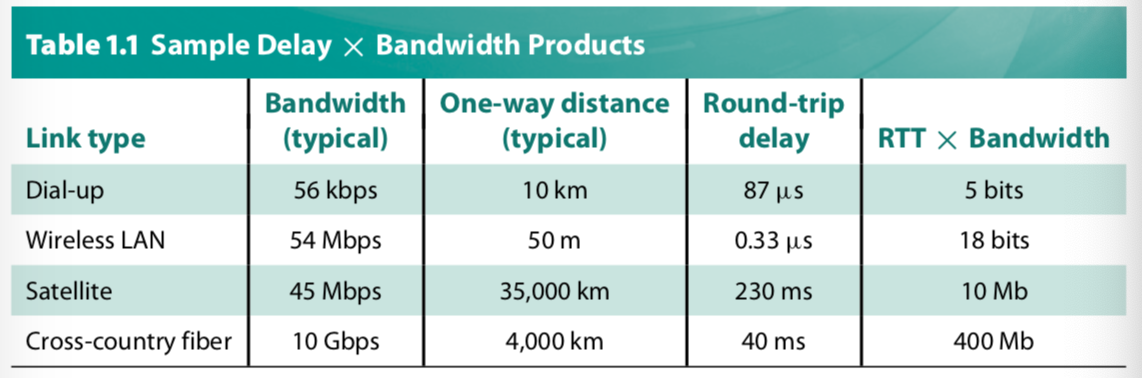
The delay×bandwidth product captures the volume of a network channel — the maximum number of bits in transit at any given instant.
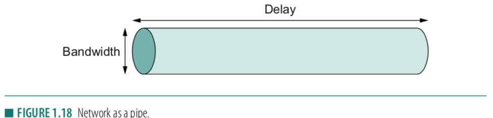
Pipe analogy: If a channel between two processes is a hollow pipe, then:
- Latency = length of the pipe
- Bandwidth = diameter of the pipe
- Delay × Bandwidth = volume of the pipe = maximum bits in flight simultaneously
2.2 Calculation
\[\text{Delay} \times \text{Bandwidth} = \text{bits in the pipe}\]Example: transcontinental channel, one-way latency = 50 ms, bandwidth = 45 Mbps:
\[50 \times 10^{-3}\ \text{s} \times 45 \times 10^6\ \text{bits/s} = 2.25 \times 10^6\ \text{bits} \approx 280\ \text{KB}\]This means the channel holds as many bytes as a personal computer’s memory from the early 1980s.
2.3 Significance: Bits in Flight
The delay×bandwidth product determines how many bits the sender must transmit before the first bit arrives at the receiver:
- Sender transmits → first bit arrives at receiver after one one-way latency
- Receiver signals back → signal arrives at sender after another one-way latency = 1 RTT total
- The sender can transmit RTT × Bandwidth bits before hearing back from the receiver
From the example above (RTT = 2 × 50 ms = 100 ms):
\[100 \times 10^{-3}\ \text{s} \times 45 \times 10^6\ \text{bits/s} = 4.5 \times 10^6\ \text{bits} \approx 548\ \text{KB}\]If the receiver signals the sender to stop, the sender may receive up to 1 RTT×bandwidth worth of data before it can respond. If the sender does not fill the pipe — does not send a full RTT×bandwidth worth of data before waiting — it will not fully utilize the network.
3. Units and Pitfalls 单位与常见误区
Two common pitfalls when working with networking units:
3.1 Bits vs Bytes
- Lowercase b = bits
- Uppercase B = bytes
- Example: 10 Mbps ≠ 10 MBps
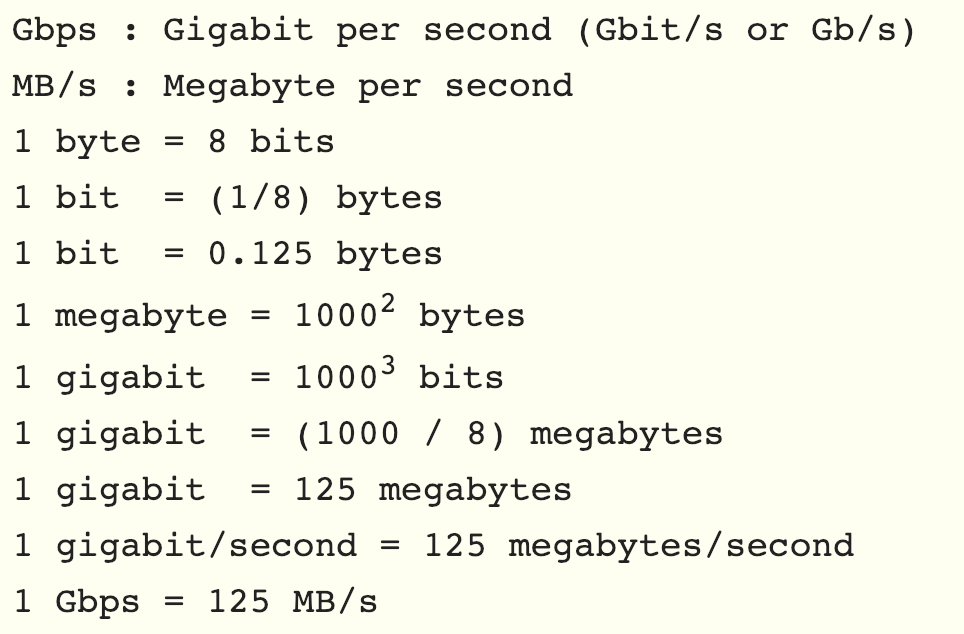
3.2 Mega (M) and Kilo (K) — Two Definitions
| Context | M means | K means |
|---|---|---|
| Network bandwidth (Mbps) | 10⁶ (governed by clock speed: 10 MHz → 10 Mbps) | 10³ |
| Memory / file sizes | 2²⁰ = 1,048,576 | 2¹⁰ = 1,024 |
Both definitions appear in networking — bandwidth is specified in powers of 10 (clock-driven), while memory and file sizes use powers of 2. This creates systematic unit confusion when calculating delay×bandwidth products.
4. High-Speed Networks 高速网络
4.1 Bandwidth Increases; Latency Does Not
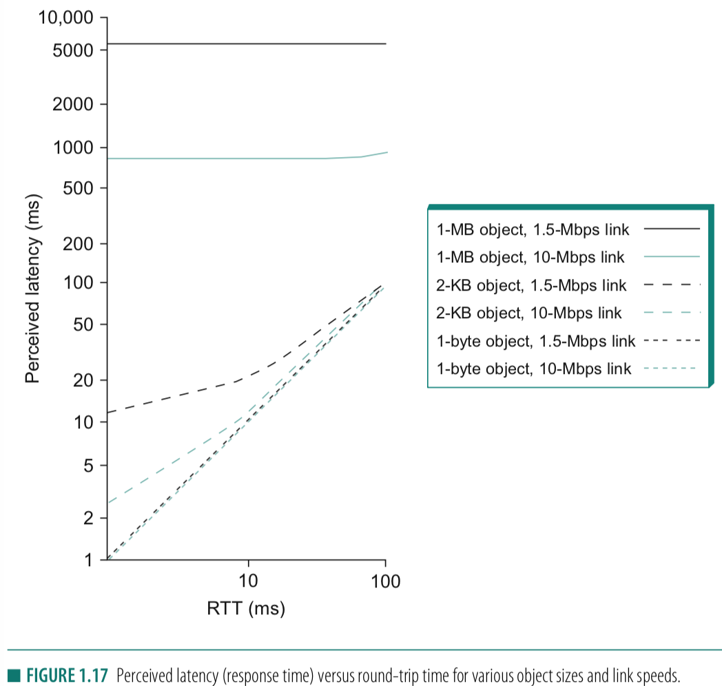
High-speed networks bring dramatically higher bandwidth, but the speed of light is fixed. In other words: “high speed” does not mean latency improves at the same rate as bandwidth.”
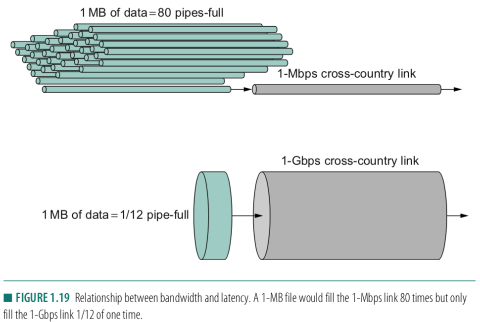
A transcontinental RTT of 100 ms is the same on a 1-Mbps link as on a 1-Gbps link.
4.2 Effect on Data Transfer
Transmitting a 1-MB file (= 8 × 10⁶ bits):
| Network | Transmit time | RTT = 100 ms | Pipe volume | File vs pipe |
|---|---|---|---|---|
| 1 Mbps | 8 s | fixed | 10⁵ bits | File = 80 pipes |
| 1 Gbps | 8 ms | fixed | 10⁸ bits | File = 0.08 pipes |
On a 1-Mbps network, the 1-MB file requires 80 RTTs to transmit (each RTT carries 1.25% of the file). On a 1-Gbps network, the entire file doesn’t even fill one RTT’s worth of pipe (delay×BW = 12.5 MB). Latency, not throughput, dominates at high speed.
4.3 Throughput Formula
\[\text{Throughput} = \frac{\text{TransferSize}}{\text{TransferTime}}\] \[\text{TransferTime} = \text{RTT} + \frac{\text{TransferSize}}{\text{Bandwidth}}\]Therefore:
\[\text{Throughput} = \frac{\text{TransferSize}}{\text{RTT} + \text{TransferSize}/\text{Bandwidth}}\]Example — 1 MB file over 1 Gbps, RTT = 100 ms:
\[\text{TransferTime} = 0.1 + \frac{8 \times 10^6}{10^9} = 0.1 + 0.008 = 0.108\ \text{s}\] \[\text{Throughput} = \frac{8 \times 10^6}{0.108} \approx 74\ \text{Mbps}\]Even with 1 Gbps of bandwidth, RTT dominance caps effective throughput far below line rate for small transfers.
5. Application Performance Needs 应用性能需求
5.1 Bandwidth Requirements
Some applications have fixed upper bounds on bandwidth rather than consuming “all available”:
Video streaming example (352 × 240 pixels, 24-bit color, 30 fps):
\[\text{Frame size} = \frac{352 \times 240 \times 24}{8} = 247.5\ \text{KB}\] \[\text{Required throughput} = 247.5 \times 10^3 \times 30 = 75\ \text{Mbps (uncompressed)}\]Providing more bandwidth than 75 Mbps is useless — the application has a fixed data rate to transmit per second.
5.2 Compressed Video and Burst Traffic
In practice, video is compressed — adjacent frames differ only slightly, and human perception does not require full detail. Compressed video does not flow at a constant rate; it varies with:
- Amount of motion and detail in the scene
- Compression algorithm in use
This means the average bandwidth requirement can be specified (e.g., 2 Mbps), but the instantaneous rate varies. An application that averages 2 Mbps over 2 seconds (1 Mb in second 1, 3 Mb in second 2) will overflow a channel engineered for exactly 2 Mb/s in any one second.
Network designers must therefore bound both the average rate and the peak burst — how many bytes can be sent at the peak rate before reverting to the average. Buffers must be sized to absorb the burst.
5.3 Jitter 抖动
Jitter: variation in inter-packet arrival times caused by variable queuing delays inside the network. Packets leave the source with uniform spacing but arrive at the sink with uneven gaps.
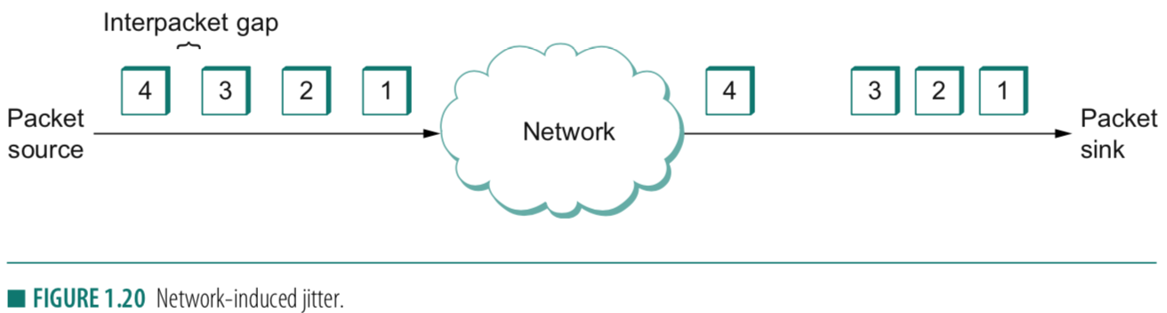
Jitter is particularly damaging to real-time applications (VoIP, streaming video) because it forces the receiver to buffer incoming data and introduce a playback delay to smooth presentation.
6. Bottleneck Analysis: I/O Bus 瓶颈分析
6.1 Key Definitions
- Memory bandwidth
: rate at which data can be read from or stored into semiconductor memory by the processor
- I/O bus
: connects the CPU to all components except RAM; moves data between components and to/from the CPU
- Bottleneck
: a point where the flow of data is impaired because there is insufficient capacity to handle current traffic volume
6.2 Workstation as Packet Switch
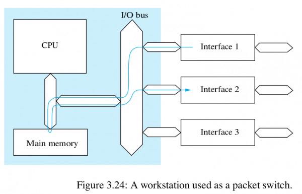
In a workstation used as a packet switch, packets arrive on a network interface, traverse the I/O bus to main memory, and then traverse the I/O bus again back to an outbound interface (via DMA). Each packet therefore crosses the I/O bus twice.
6.3 Interface Count Calculation
Since I/O bus speed < memory bandwidth, the I/O bus is the bottleneck.
\[\text{Effective bandwidth} = \frac{\text{I/O bus bandwidth}}{2}\]Example: I/O bus = 1000 Mbps, each interface = 100 Mbps:
\[\text{Effective bandwidth} = \frac{1000}{2} = 500\ \text{Mbps}\] \[\text{Number of interfaces} = \left\lfloor \frac{500}{100} \right\rfloor = 5\]Key Takeaways
- Bandwidth
= data rate (bps); latency = end-to-end travel time. Both must be measured and managed independently.
- Three latency components
: propagation (speed of light), transmission (size/bandwidth), queuing (switch buffering).
- Delay×Bandwidth product
= volume of the pipe = maximum bits in transit simultaneously; the sender must keep the pipe full to maximize utilization.
- At high speed
, bandwidth grows but latency is fixed by the speed of light — latency dominates for small transfers, making RTT the binding constraint.
- Throughput formula
:
TransferSize / (RTT + TransferSize/Bandwidth)— RTT dominates whenTransferSize/Bandwidth ≪ RTT. - M = 10⁶ in networking
(clock-driven), but M = 2²⁰ for memory — mixing the two causes systematic calculation errors.
- Video bandwidth
=
(width × height × color depth / 8) × fps; compressed video has variable burst rate, requiring both average and peak bound specification. - Jitter
degrades real-time applications — receivers must buffer and introduce playback delay to smooth variable inter-packet arrival.
- I/O bus bottleneck
: each packet crosses the bus twice (DMA in + out), so effective throughput = I/O bus bandwidth / 2.
References
- Computer Networks: A Systems Approach — Peterson & Davie, Chapter 1 (Foundation)
- CS 528 Computer Networks — Lecture notes: 1.5 Performance
Comments powered by Disqus.